What Can Differentiability Do for Density Functional Theory

So what can Automatic Differentiation (AD) do for Density Functional Theory? The short answer is that AD can greatly simplify the calculation of all gradients. Researchers don’t have to manually derive all the gradients or Hessian matrices and implement them on their own – you can just write down the function that you would like to differentiate, and AD will do the rest.

Next, we will show two examples to demonstrate how AD can help us calculate the Kohn-Sham Hamiltonian matrix and the Ewald energy.

Example: Kohn-Sham Hamiltonian matrix

Once we have a ground-state density \(\rho(\mathbf{r})\), the Kohn-Sham Hamiltonian matrix is defined as

\[H_{ij} = < \psi_i | \hat{H}[\rho] | \psi_j >\]

where \(\psi_i\) is the Kohn-Sham orbital. Although the analytical form of such a matrix is available, we don’t have to implement it on our own, which could be quite time-consuming. As long as we have the total energy functional, we can use AD to calculate the Hamiltonian matrix, as we know that it is simply the Hessian of the total energy functional with respect to the orbital coefficients.

Let \(\mathbf{u}\) be a coefficient vector of the Kohn-Sham orbitals, and a linear combination of the orbitals can be written as:

\[\chi = \sum_i u_i \psi_i\]

The expectation of the Hamiltonian with respect to the linear combination is:

\[E = < \chi | \hat{H}[\rho] | \chi > = \sum_{ij} u_i^* u_j < \psi_i | \hat{H}[\rho] | \psi_j > = \mathbf{u}^\dagger H \mathbf{u}\]

Therefore, we can obtain the Hamiltonian matrix \(H\) by calculating the Hessian of the total energy functional with respect to the orbital coefficients \(\mathbf{u}\).

\[\dfrac12 \nabla_{\mathbf{u}}^2 E = H\]

Well, it is not as simple as it looks. The above energy function, which is a complex-valued function, is not a holomorphic function with respect to the orbital coefficients. Currently, JAX does not support the API of Hessian for complex-valued non-holomorphic functions. Therefore, we need to implement a complex-Hessian function using the jax.vjp function. This implementation is now available in the jrystal.hessian.complex_hessian function.

If you understand the above derivation, you can understand how we implement the jrystal.hamiltonian.hamiltonian_matrix function.

def hamiltonian_matrix(
  coeff,
  positions,
  charges,
  effictive_density_grid,
  g_vector_grid,
  k,
  vol,
  xc
):

  num_bands = coeff.shape[2]

  def efun(u):
    _coeff = jnp.einsum("i, *n i a b c -> *n a b c", u, coeff)
    _coeff = jnp.expand_dims(_coeff, axis=-4)

    energy = hamiltonian_matrix_trace(
      _coeff,
      positions,
      charges,
      effictive_density_grid,
      g_vector_grid,
      k,
      vol,
      xc,
      kohn_sham,
    )

    return 0.5 * jnp.sum(energy)

  x = jnp.ones(num_bands, dtype=band_coefficient.dtype)
  return complex_hessian(efun, x)

Example: DFT forces

The DFT force acting on an ion A is defined as:

\[F_A = - \nabla_A E_{\text{tot}}[\rho](A)\]

where \(A\) is the position of the ion.

In jrystal, we can calculate the force using the jax.grad function.

Initialize the system and prepare the mesh grids and other parameters.

import jax
import jax.numpy as jnp
import jrystal as jr
from jrystal import energy

key = jax.random.PRNGKey(123)
charges = jnp.array([6, 6])  # two carbon atoms
positions = jnp.array([[-0.8425, -0.8425, -0.8425], [0.8425, 0.8425, 0.8425]])
cell_vectors = jnp.array([[0., 3.37, 3.37], [3.37, 0., 3.37], [3.37, 3.37, 0.]])

crystal = jr.Crystal(chages=charges, positions=positions, cell_vectors=cell_vectors)

# Set grid parameters
grid_size = [64, 64, 64]  # Real and reciprocal space grid
kpt_grid = [1, 1, 1]      # Gamma point

g_vecs = jr.grid.g_vectors(crystal.cell_vectors, grid_sizes=grid_size)
kpts = jr.grid.k_vectors(crystal.cell_vectors, grid_sizes=kpt_grid)

freq_mask = jr.grid.spherical_mask(
    cell_vectors=crystal.cell_vectors,
    grid_sizes=grid_size,
    cutoff_energy=100
)

# Set the occupation
occ = jr.occupation.uniform(num_kpts, crystal.num_electron, num_bands=num_bands)
density = jr.pw.density_grid(coeff, crystal.vol, occ)

We can define a energy function of the positions of the ions. using the jrystal.energy.total_energy function.

def energy(position):
  e_tot = jr.energy.total_energy(coeff, position, crystal.charges, g_vecs, kpts, crystal.vol, occ)
  e_nuc = jr.energy.nuclear_repulsion(position, crystal.charges, crystal.cell_vectors, g_vecs, crystal.vol, 0.1, 5000)
  return (e_tot + e_nuc)

The forces of the ions are the negative gradient of the energy function with respect to the positions of the ions.

 forces = -jax.grad(energy)(positions)
 print(forces)

 >>> [[ 2.4587612  2.4767363  2.3396077]
[-2.4314194 -2.5411198 -2.3505976]]

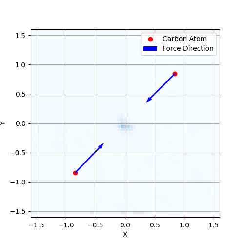
The next figure shows the forces calculated by jrystal on a diamond crystal with almost uniformly distributed electron density. The forces are calculated using jax.grad and jrystal.