The rapid adoption of text-to-image diffusion models in society underscores an urgent need to address their biases. Without interventions, these biases could propagate a skewed worldview and restrict opportunities for minority groups. In this work, we frame fairness as a distributional alignment problem. Our solution consists of two main technical contributions: (1) a distributional alignment loss that steers specific characteristics of the generated images towards a user-defined target distribution, and (2) adjusted direct finetuning of diffusion model's sampling process (adjusted DFT), which leverages an adjusted gradient to directly optimize losses defined on the generated images. Empirically, our method markedly reduces gender, racial, and their intersectional biases for occupational prompts. Gender bias is significantly reduced even when finetuning just five soft tokens. Crucially, our method supports diverse perspectives of fairness beyond absolute equality, which is demonstrated by controlling age to a 75% young and 25% old distribution while simultaneously debiasing gender and race. Finally, our method is scalable: it can debias multiple concepts at once by simply including these prompts in the finetuning data.
Method: Distributional Alignment Loss
Consider we want to control a categorical attribute of the generated images that has \(K\) classes and align it towards a target distribution \(\mathcal{D}\). Each class is represented as a one-hot vector of length \(K\) and \(\mathcal{D}\) is a discrete distribution over these vectors (or simply points). We first generate a batch of images \(\mathcal{I}=\{\boldsymbol{x}^{(i)}\}_{i\in[N]}\) using the finetuned diffusion model and some prompt P. For every generated image \(\boldsymbol{x}^{(i)}\), we use a pre-trained classifier \(h\) to produce a class probability vector \(\boldsymbol{p}^{(i)}=[p_{1}^{(i)},\cdots,p_{K}^{(i)}]=h(\boldsymbol{x}^{(i)})\), with \(p_{k}^{(i)}\) denoting the estimated probability that \(\boldsymbol{x}^{(i)}\) is from class \(k\). Assume we have another set of vectors \(\{\boldsymbol{u}^{(i)}\}_{i\in[N]}\) that represents the target distribution and where every \(\boldsymbol{u}^{(i)}\) is a one-hot vector representing a class, we can compute the optimal transport (OT) from \(\{\boldsymbol{p}^{(i)}\}_{i\in[N]}\) to \(\{\boldsymbol{u}^{(i)}\}_{i\in[N]}\):
$$ \sigma^* = {\arg\min}_{\sigma\in \mathcal{S}_{N}}\sum_{i=1}^{N}|\boldsymbol{p}^{(i)}-\boldsymbol{u}^{(\sigma_{i})}|_{2}\textrm{,}$$
where \(\mathcal{S}_{N}\) denotes all permutations of \([N]\), \(\sigma=[\sigma_1,\cdots,\sigma_N]\), and \(\sigma_i\in[N]\). Intuitively, \(\sigma^*\) finds, in the class probability space, the most efficient modification of the current images to match the target distribution.
We construct \(\{\boldsymbol{u}^{(i)}\}_{i\in[N]}\) to be iid samples from the target distribution and compute the expectation of OT:
$$\boldsymbol{q}^{(i)} = \mathbb{E}_{\boldsymbol{u}^{(1)},\cdots,\boldsymbol{u}^{(N)} \sim \mathcal{D}} ~ [\boldsymbol{u}^{(\sigma^*_{i})}],~\forall i\in[N] \textrm{.} $$
\(\boldsymbol{q}^{(i)}\) is a probability vector where the \(k\)-th element is the probability that \(\boldsymbol{x}^{(i)}\) should have target class \(k\), had the batch of generated images indeed followed the target distribution \(\mathcal{D}\). The expectation of OT can be computed analytically when the number of classes \(K\) is small or approximated by empirical average when \(K\) increases. We note one can also construct a fixed set of \(\{\boldsymbol{u}^{(i)}\}_{i\in[N]}\), for example half male and half female to represent a balanced gender distribution. But this construction poses a stronger finite-sample alignment objective and neglects the sensitivity of OT.
Finally, we generate target classes \(y^{(1)},\cdots,y^{(N)}\in [K]\) and confidence of these targets \(c^{(1)},\cdots,c^{(N)}\in [0,1]\) by: \(y^{(i)} = \arg\max(\boldsymbol{q}^{(i)}), c^{(i)} = \max(\boldsymbol{q}^{(i)})\textrm{,}\) \(\forall i\in[N]\). We define DAL as the cross-entropy loss w.r.t. these dynamically generated targets, with a confidence threshold \(C\),
$$ \mathcal{L}_{\textrm{align}} = \frac{1}{N}\sum_{i=1}^{N} \mathbb{1}[c^{(i)}\geq C] \mathcal{L}_{\textrm{CE}}(h(\boldsymbol{x}^{(i)}),y^{(i)})\textrm{.} $$
Besides DAL, we additionally regularize CLIP and DINO similarities between images generated by the original and finetuned models to preserve image semantics.
Method: Adjusted Direct Finetuning
While most diffusion finetuning methods use the same denoising diffusion loss from pre-training, Direct Finetuning (DFT) aims to directly finetune the diffusion model's sampling process to minimize any loss defined on the generated images, such as ours. We show the naive DFT, which computes the exact gradient of the sampling process, has exploding norm and variances and therefore is ineffective. Adjusted DFT leverages an adjusted gradient to overcome these issues. It opens venues for more refined and targeted diffusion model finetuning and can be applied for objectives beyond fairness. Read Section 4.2 in paper for details.
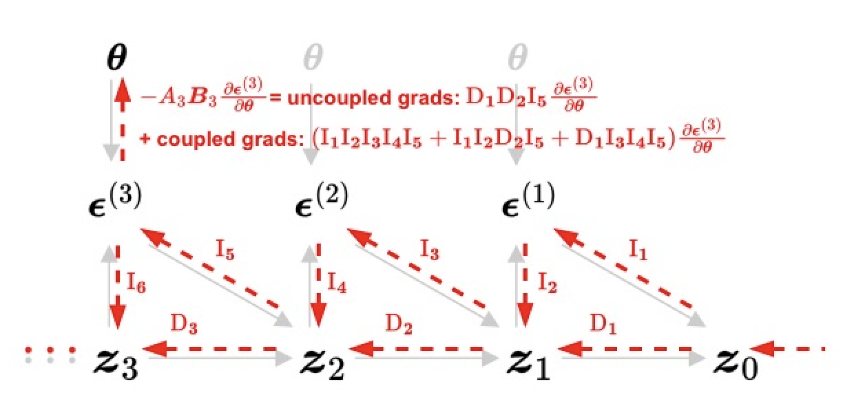
Naive DFT
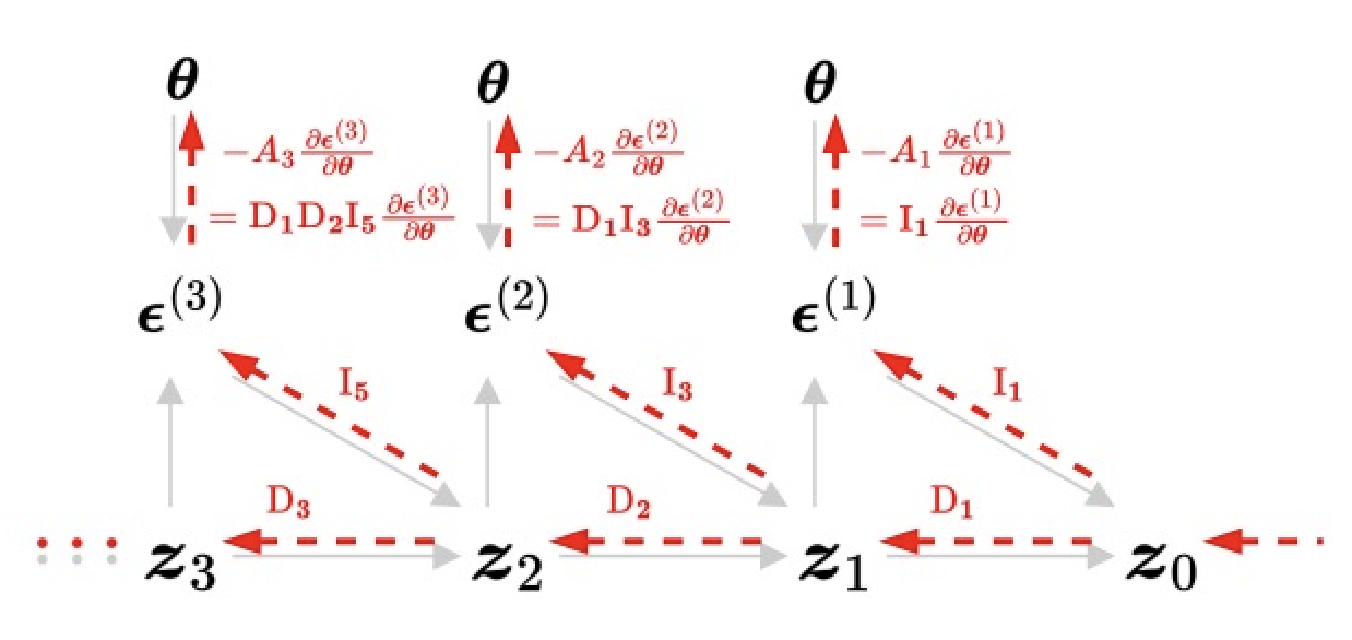
Adjusted DFT, which also standardize \(A_i\) to 1
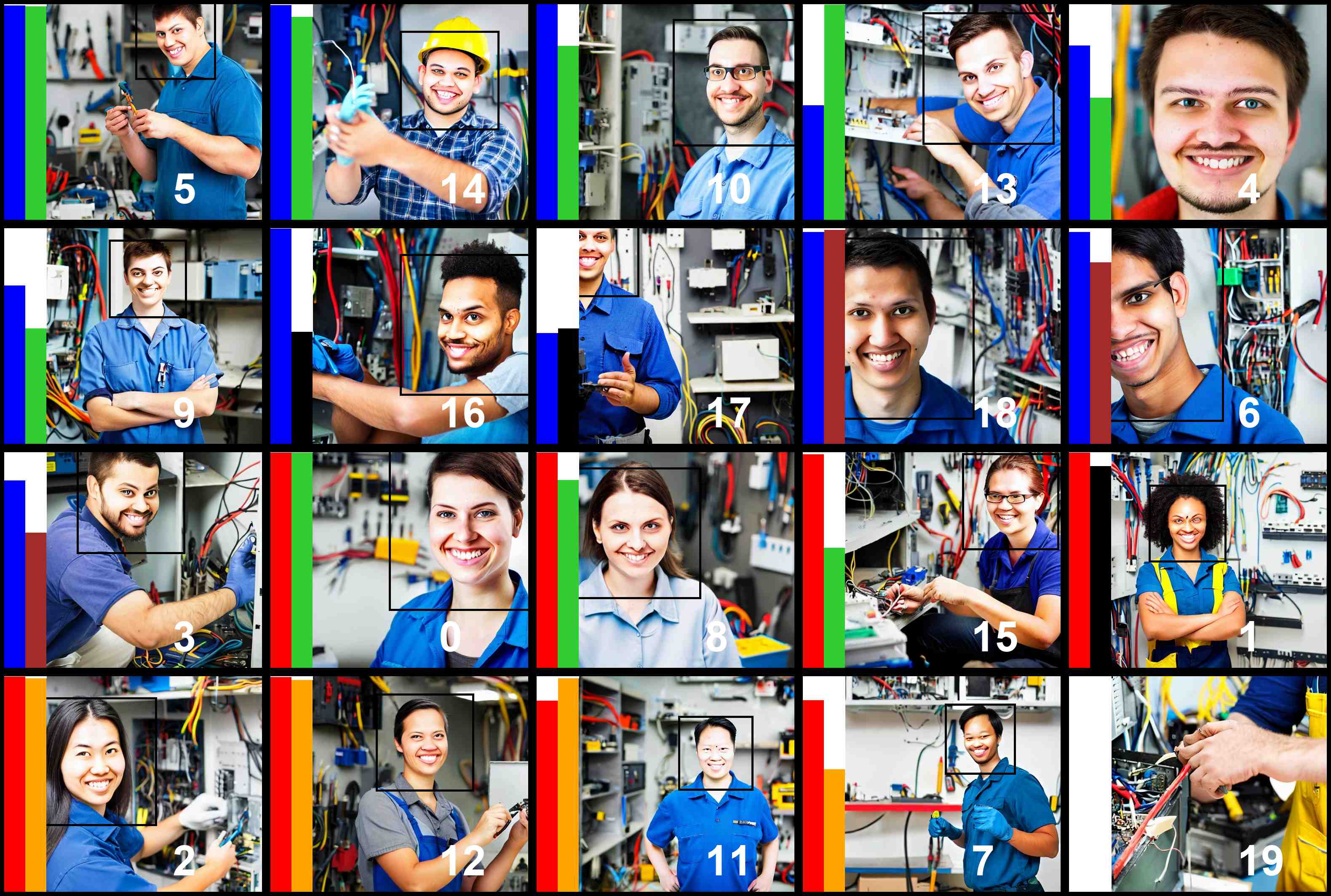
Comparison of naive and adjusted DFT of the diffusion model. Gray solid lines denote the sampling process. Red dashed lines highlight the gradient computation w.r.t. the model parameter (\(\boldsymbol{\theta}\)). Variables \(\boldsymbol{z}_{t}\) and \(\boldsymbol{\epsilon}^{(t)}\) represent data and noise prediction at time step \(t\). \(\textrm{D}_i\) and \(\textrm{I}_i\) denote the direct and indirect gradient paths between data of adjacent time steps. For instance, at \(t=3\), naive DFT computes the exact gradient \(-A_3\boldsymbol{B}_3\frac{\partial\boldsymbol{\epsilon}^{(3)}}{\partial\boldsymbol{\theta}}\) (defined in Eq. 9 in paper), which involve other time step's noise predictions (through the gradient paths \(\textrm{I}_1\textrm{I}_2\textrm{I}_3\textrm{I}_4\textrm{I}_5\), \(\textrm{I}_1\textrm{I}_2\textrm{D}_2\textrm{I}_5\), and \(\textrm{D}_1\textrm{I}_3\textrm{I}_4\textrm{I}_5\)). Adjusted DFT leverages an adjusted gradient, which removes the coupling with other time steps and standardizes \(A_i\) to 1, for more effective finetuning.
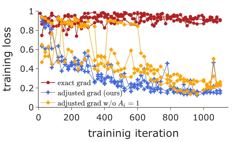
Training loss for minimizing avg CLIP & DINO similarity
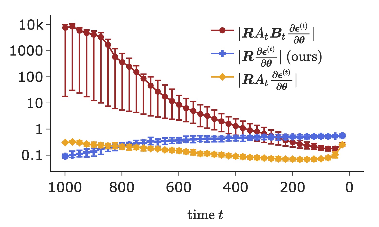
Estimated gradient scale at different time steps
The left figure plots the training loss during DFT, w/ three distinct gradients. Each reported w/ 3 random runs. The right figure estimates the scale of these gradients at different time steps. Mean and \(90\%\) CI are computed from 20 random runs. Naive DFT uses the exact gradient, whose norm is illustrated by the "\(|\boldsymbol{R}_tA_t\boldsymbol{B}_t\frac{\partial\boldsymbol{\epsilon}^{(t)}}{\partial\boldsymbol{\theta}}|\)" entry in the right figure. The proposed adjusted DFT is denoted as "ours" entry.
Results: Debiasing Gender & Race for Occupational Prompts
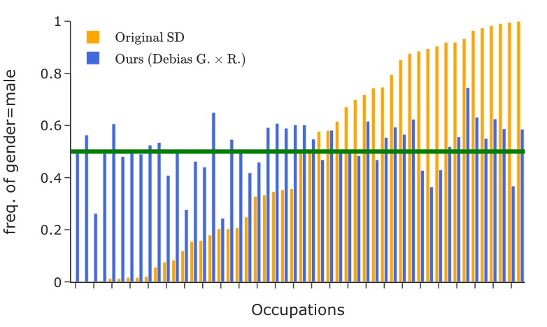
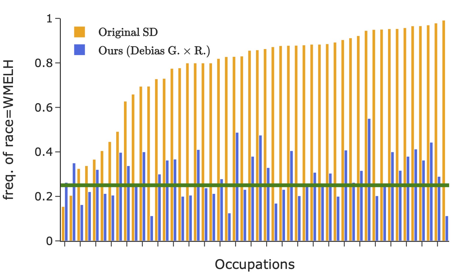
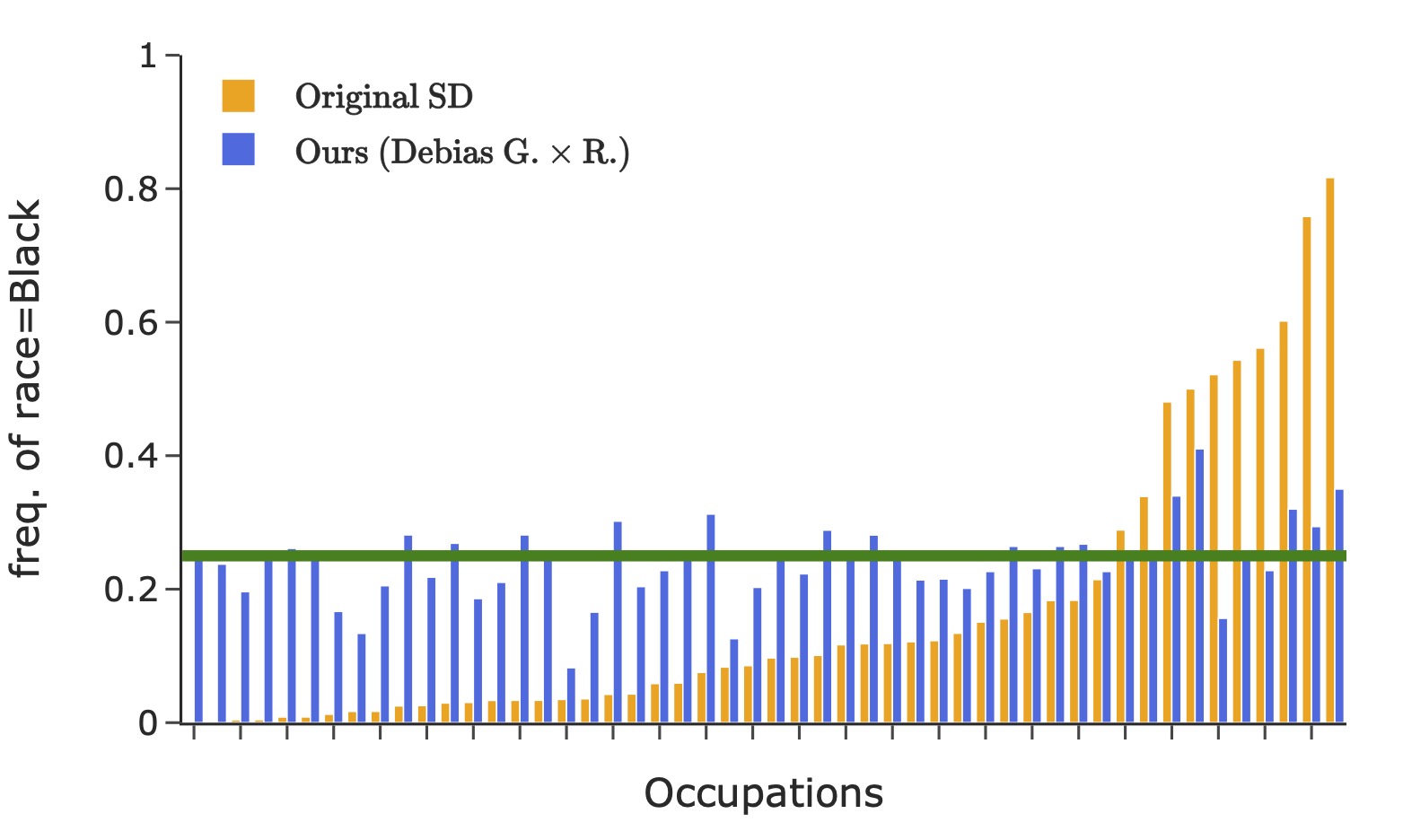
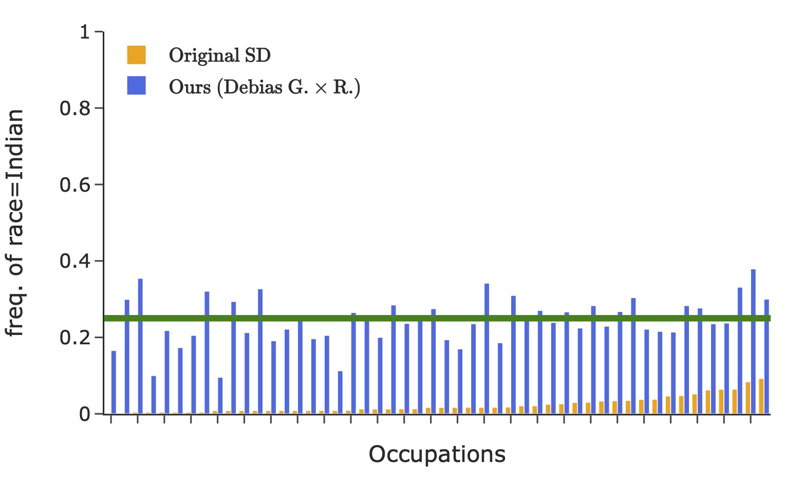
Here we debias stable-diffusion v1-5 for the intersection of gender and race, by finetuning LoRA with rank 50 applied on the text encoder. We consider binary gender and four race classes: WMELH, Asian, Black, and Indian. WMELH encompasses White, Middle Eastern, and Latino Hispanic. The prompt is contructed using the template "a photo of the face of a {occupation}, a person". We use 1000 occupations for debiasing finetuning.
For every prompt P, we compute the following metric: \(\textrm{bias}(\texttt{P}) = \frac{1}{K(K-1)/2}\sum_{i,j\in[K]:i< j} |\textrm{freq}(i)-\textrm{freq}(j)| \),
where \(\textrm{freq}(i)\) is group \(i\)'s frequency in the generated images. The number of groups \(K\) is 2/4/8 for gender/race/their intersection. The classification of an image into a specific group is based on the face that covers the largest area. This bias metric considers a perfectly balanced target distribution. It measures the disparity of different groups' representations, averaged across all contrasting groups.
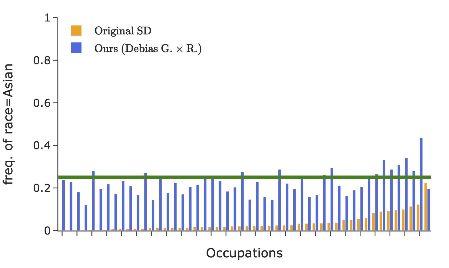
Representation of gender (the left figure) and race (the right four figures) in images generated using 50 occupational test prompts (x-axis). The green horizontal lines denote the desired target distribution.
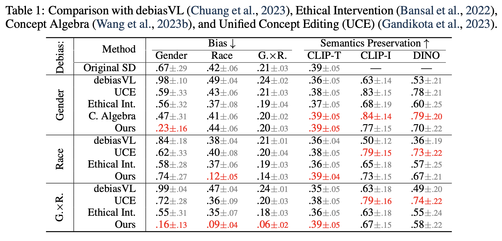
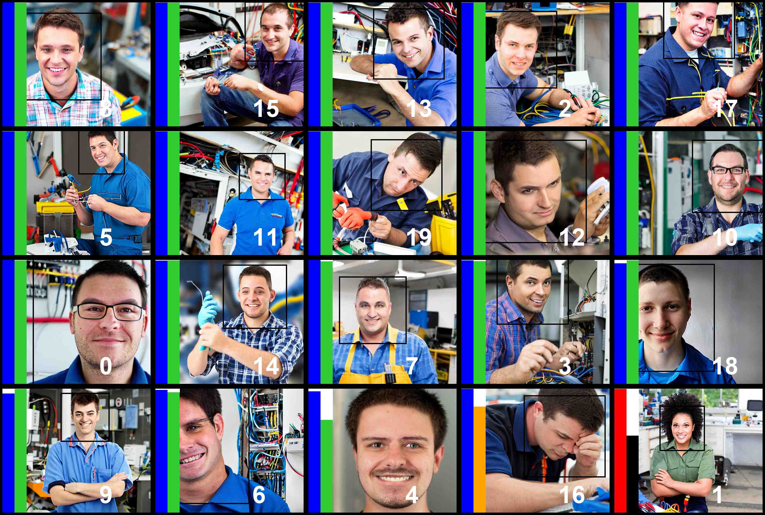
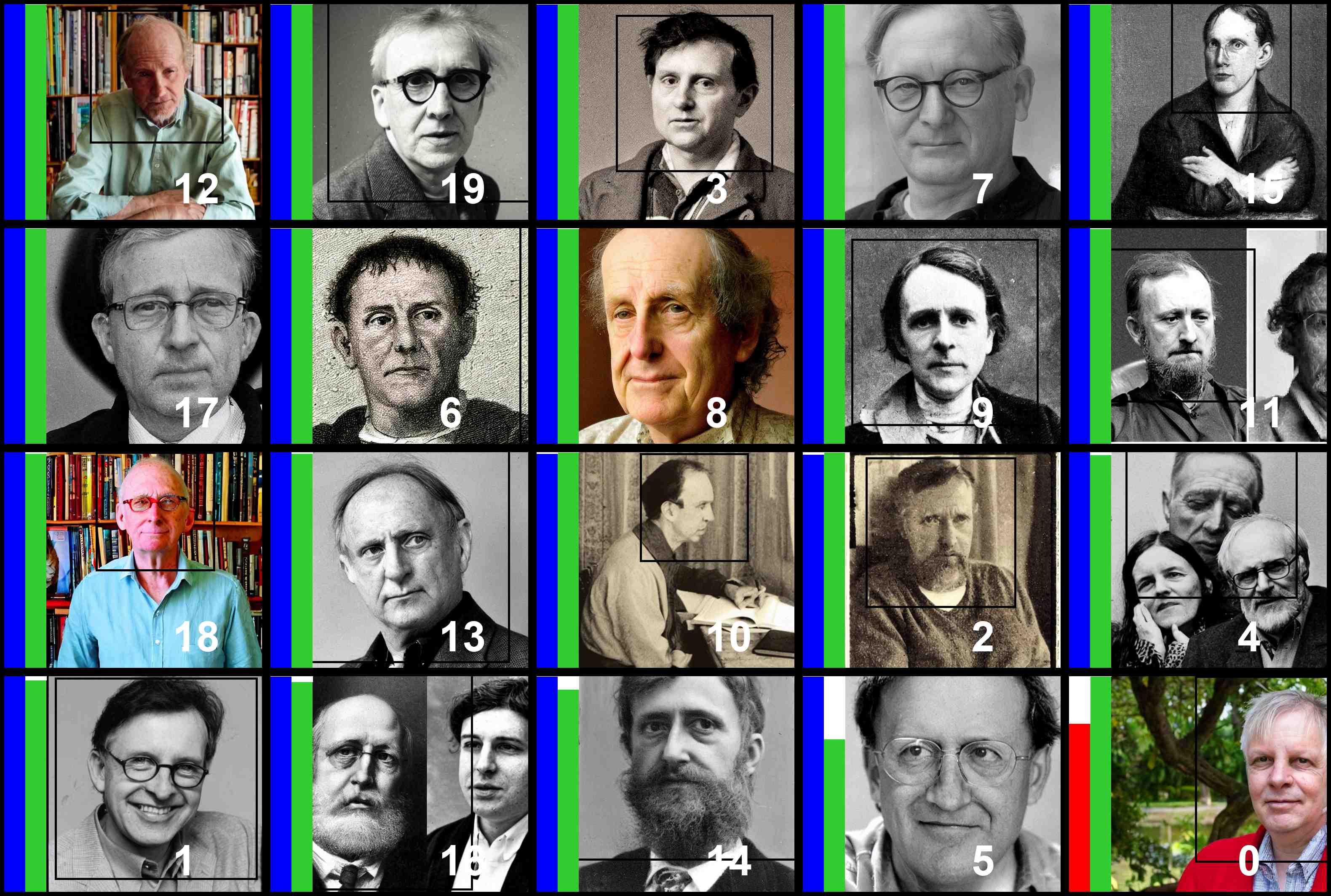
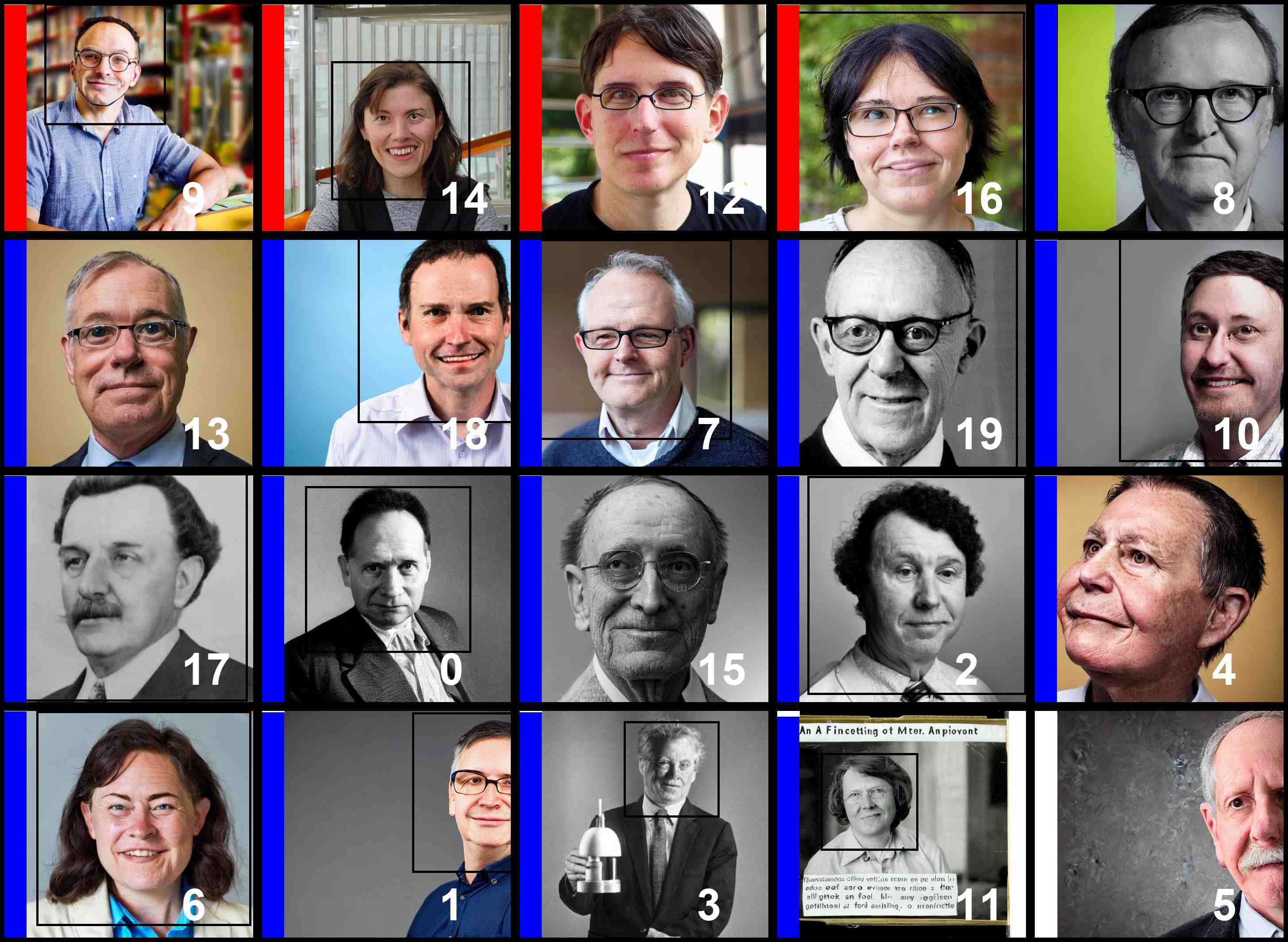
Prompt: "a photo of the face of a electrical and electronics repairer, a person". Gender bias: 0.84 (original) \(\rightarrow\) 0.11 (debiased). Racial bias: 0.48 \(\rightarrow\) 0.10. Gender\(\times\)Race bias: 0.24 \(\rightarrow\) 0.06.
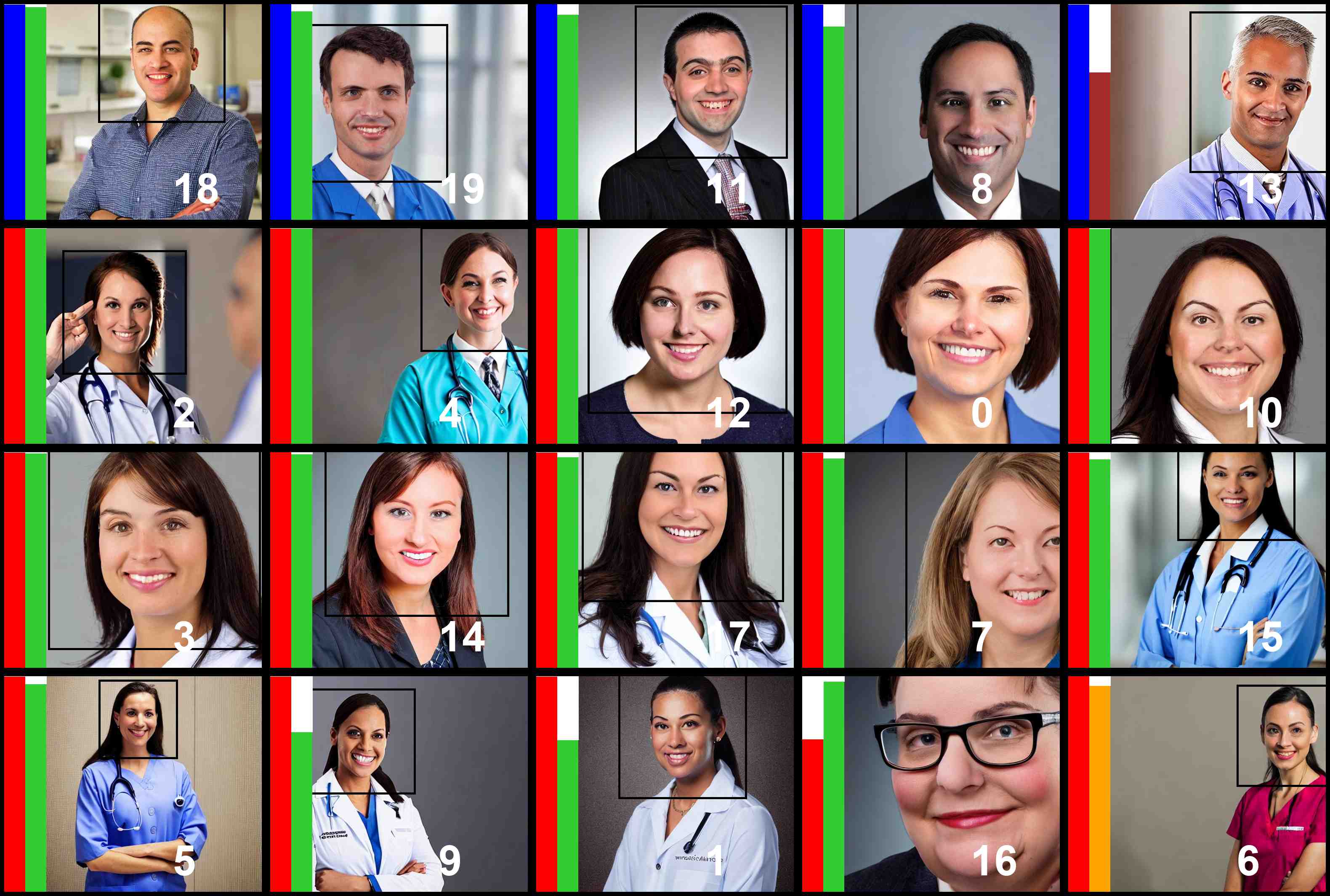
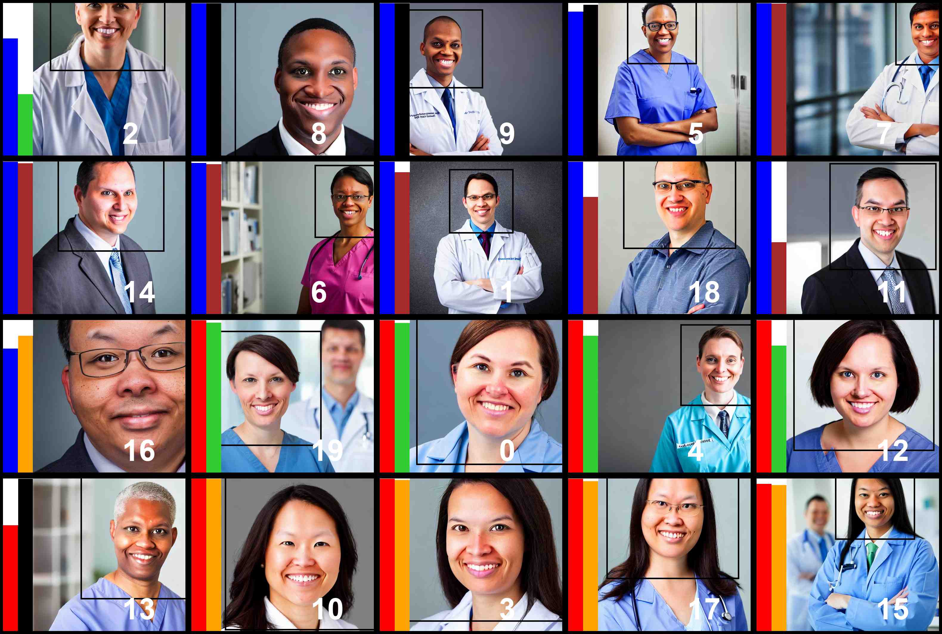
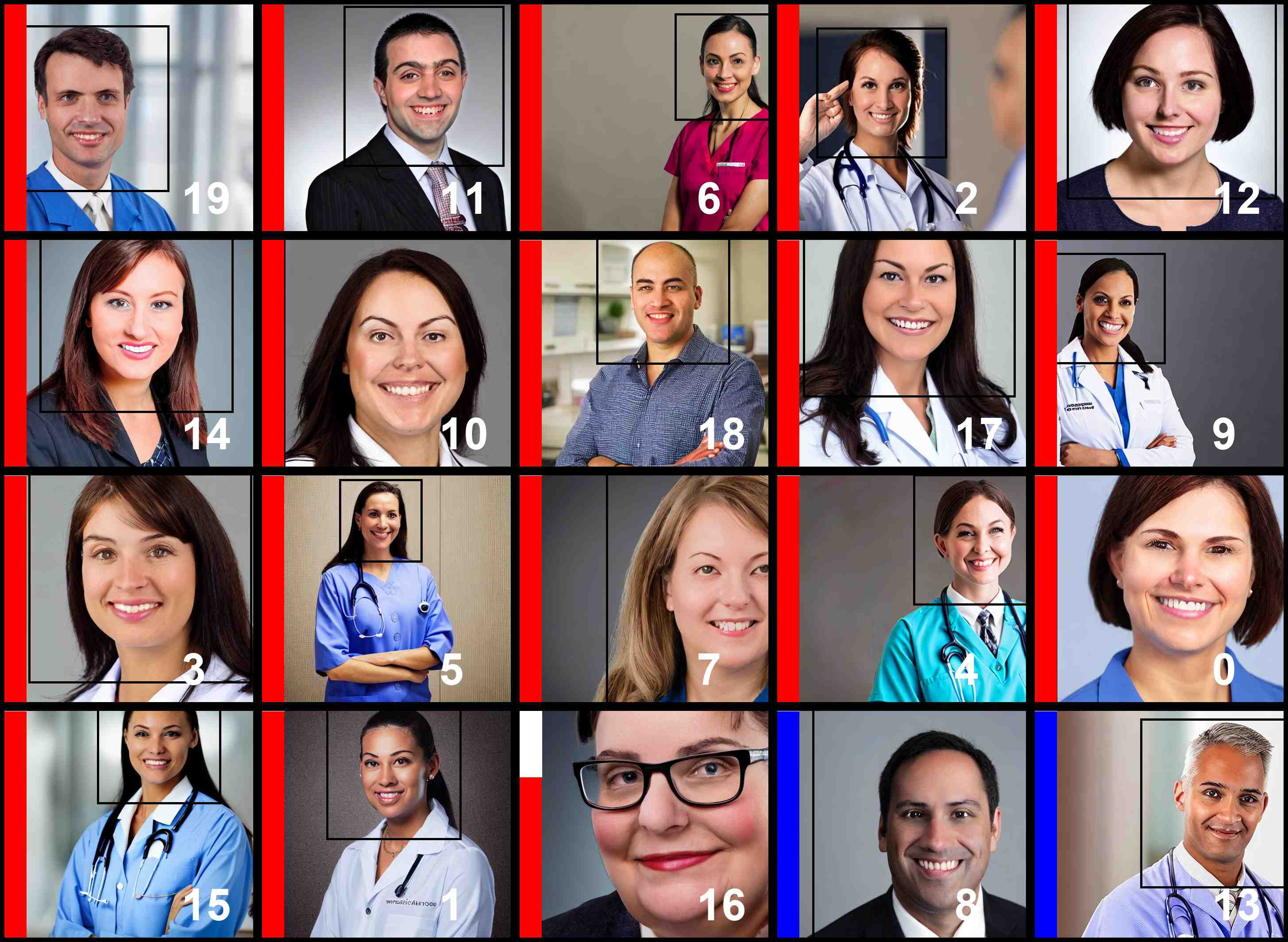
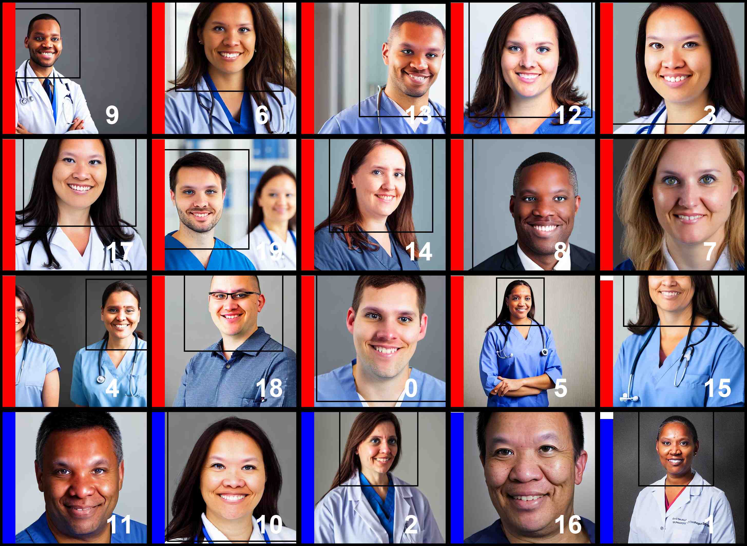
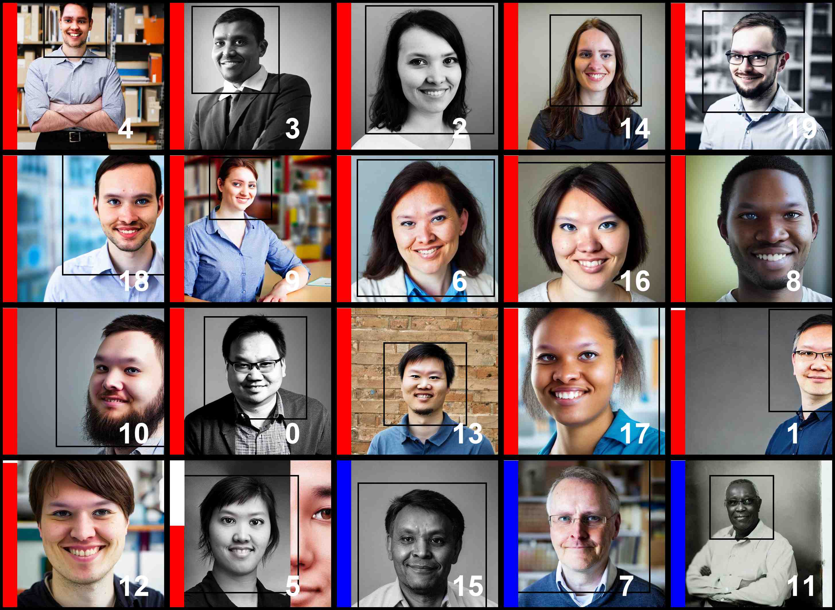
Prompt: "a photo of the face of a cardiologist, a person". Gender bias: 0 (original) \(\rightarrow\) 0.10 (debiased). Racial bias: 0.44 \(\rightarrow\) 0.08. Gender\(\times\)Race bias: 0.19 \(\rightarrow\) 0.06.
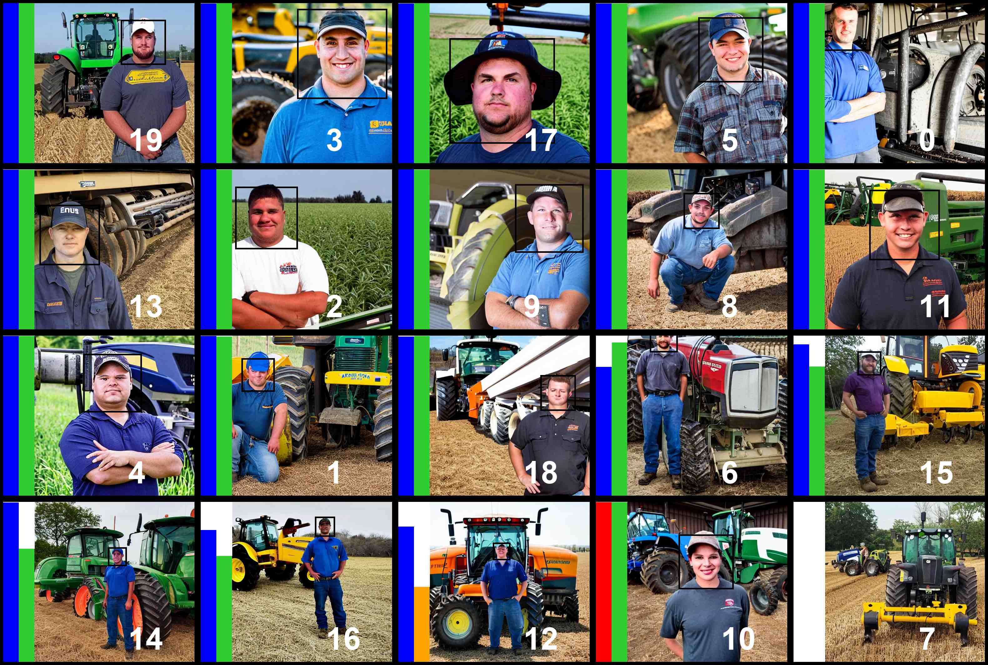
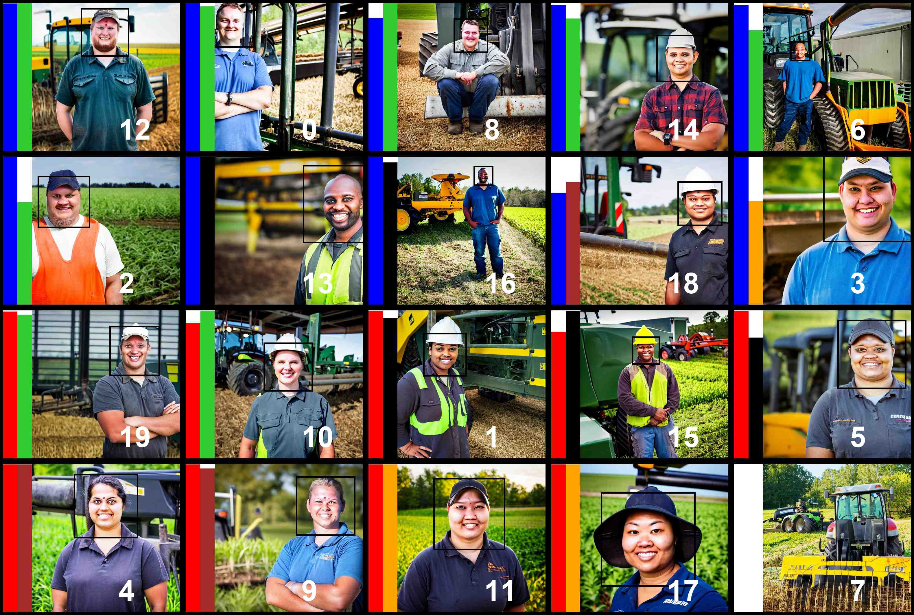
Prompt: "a photo of the face of a farm equipment service technician, a person". Gender bias: 0.95 (original) \(\rightarrow\) 0.10 (debiased). Racial bias: 0.48 \(\rightarrow\) 0.11. Gender\(\times\)Race bias: 0.24\(\rightarrow\) 0.06.
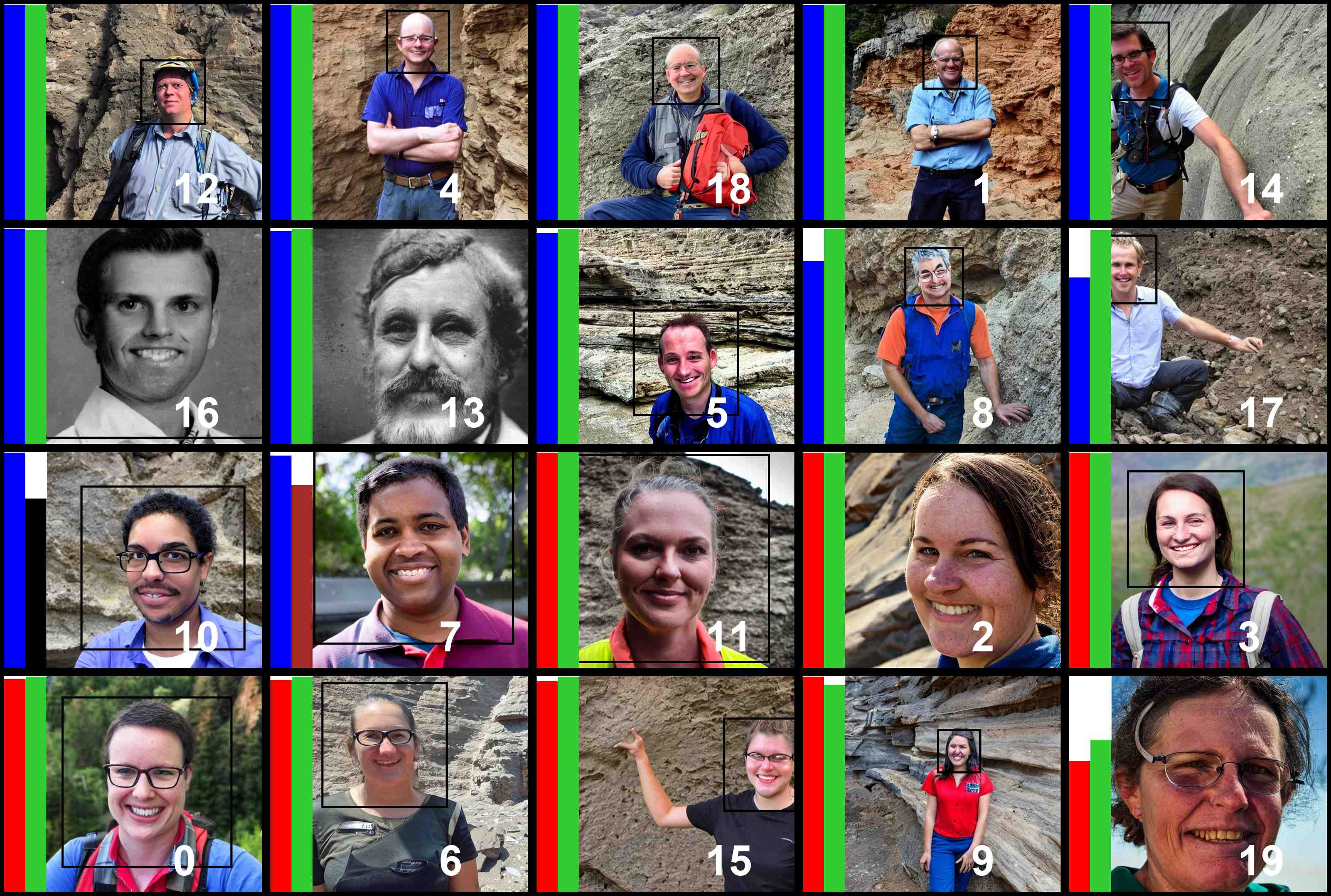
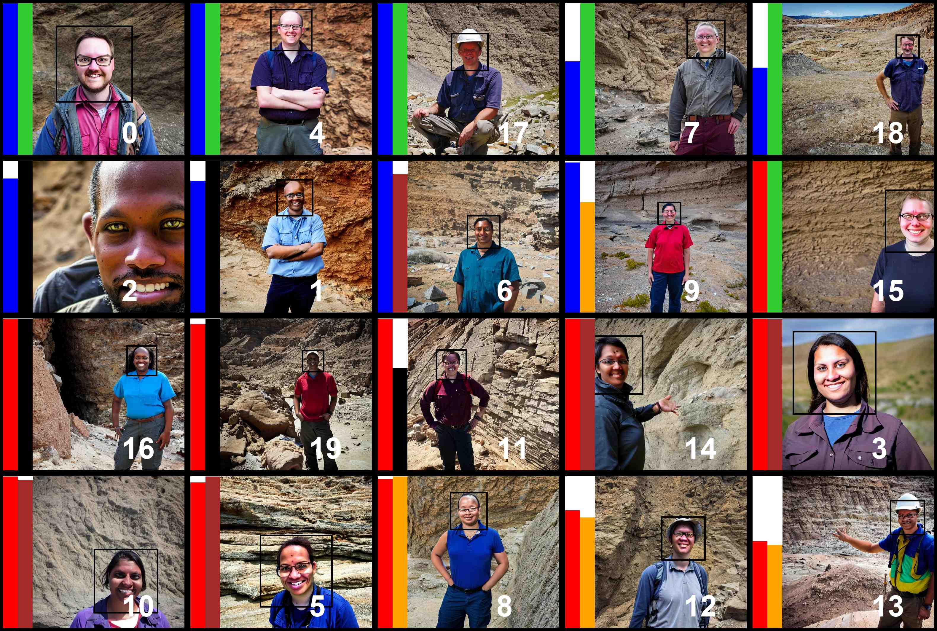
Prompt: "a photo of the face of a geologist, a person". Gender bias: 0.23 (original) \(\rightarrow\) 0.01 (debiased). Racial bias: 0.47 \(\rightarrow\) 0.11. Gender\(\times\)Race bias: 0.21 \(\rightarrow\) 0.06.
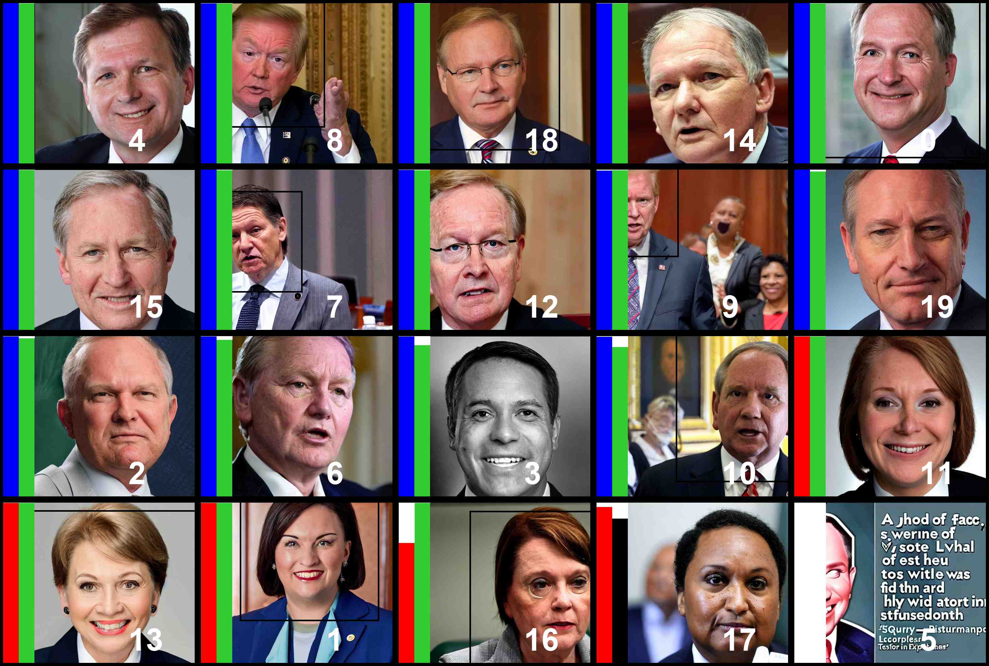
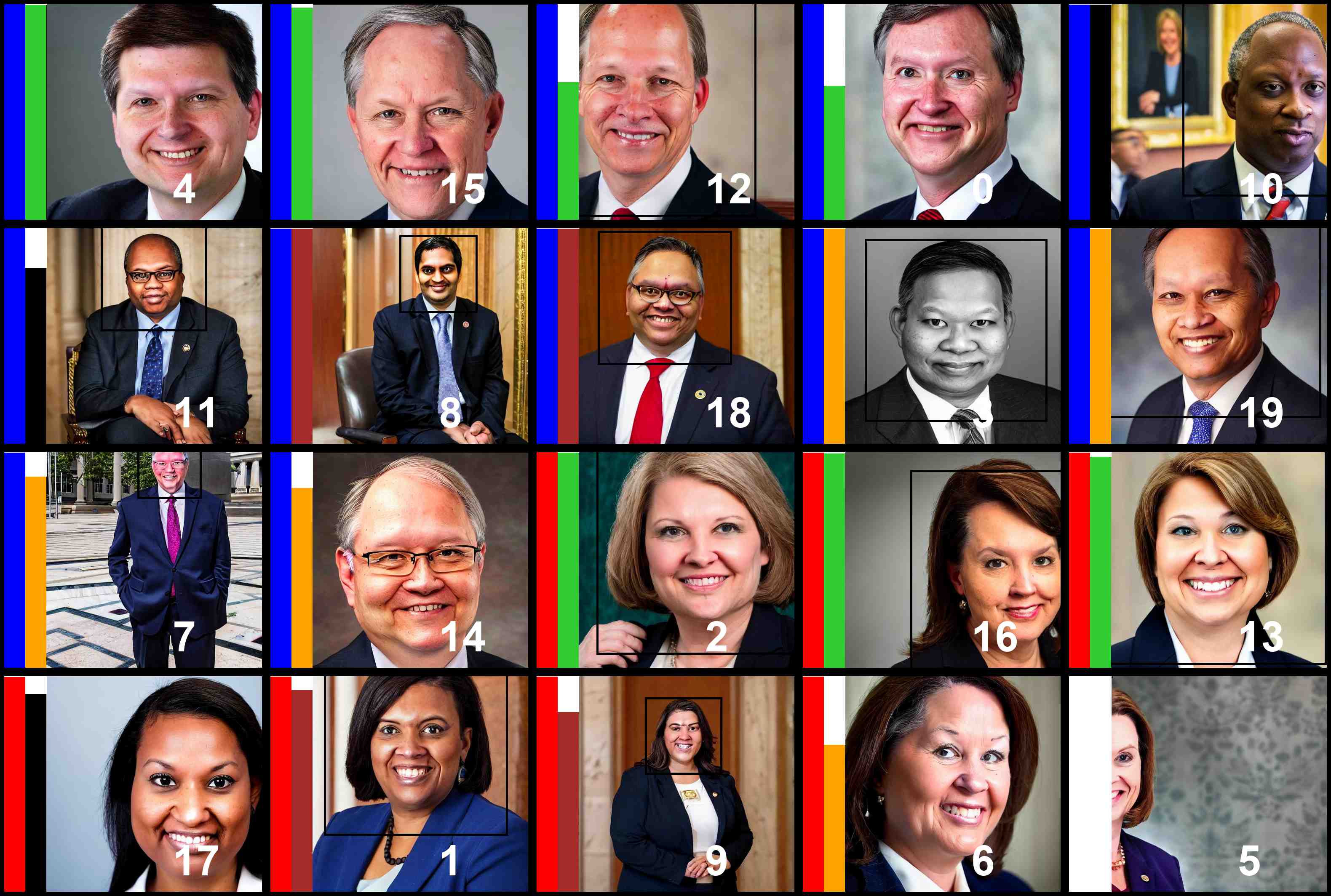
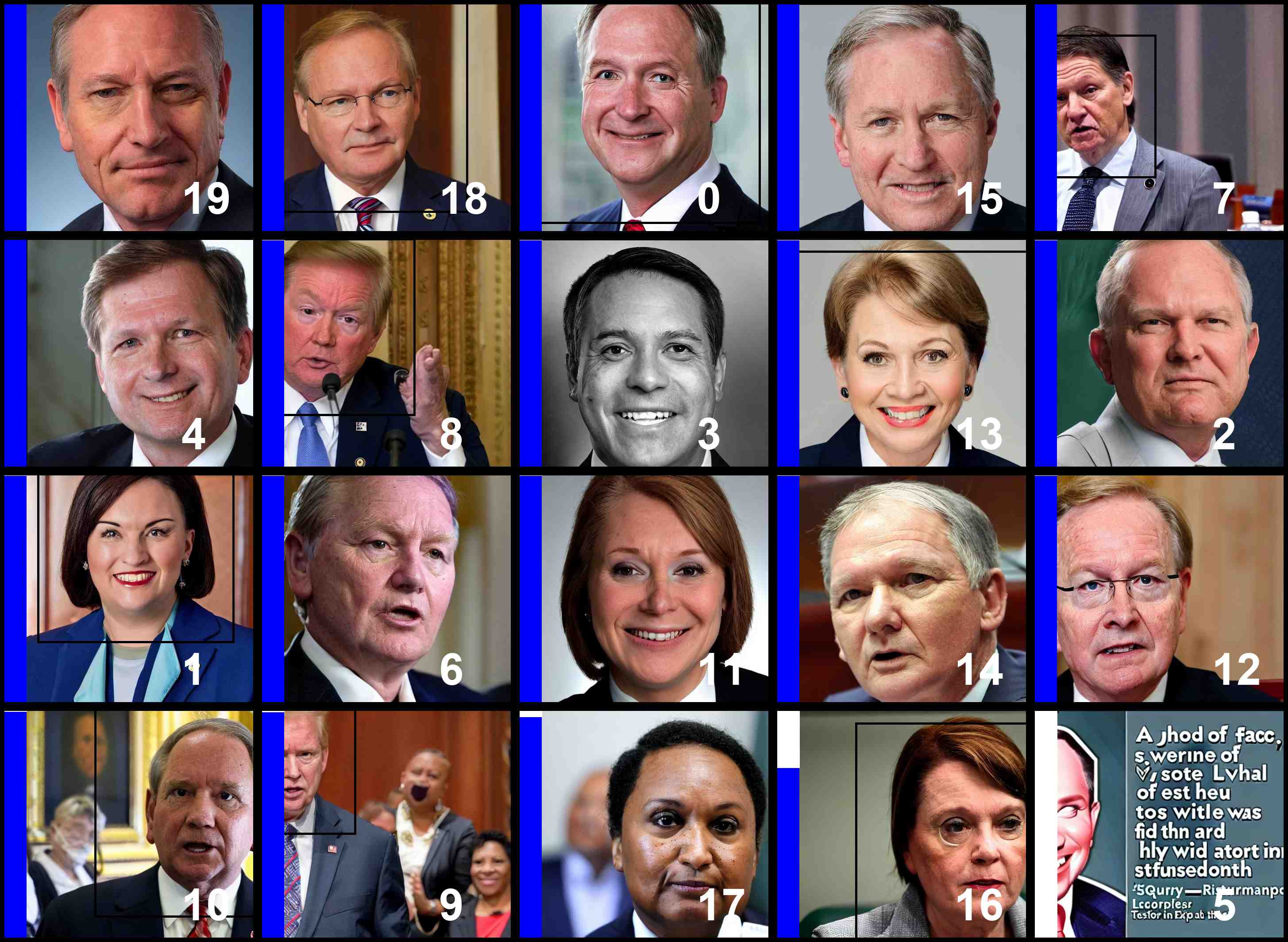
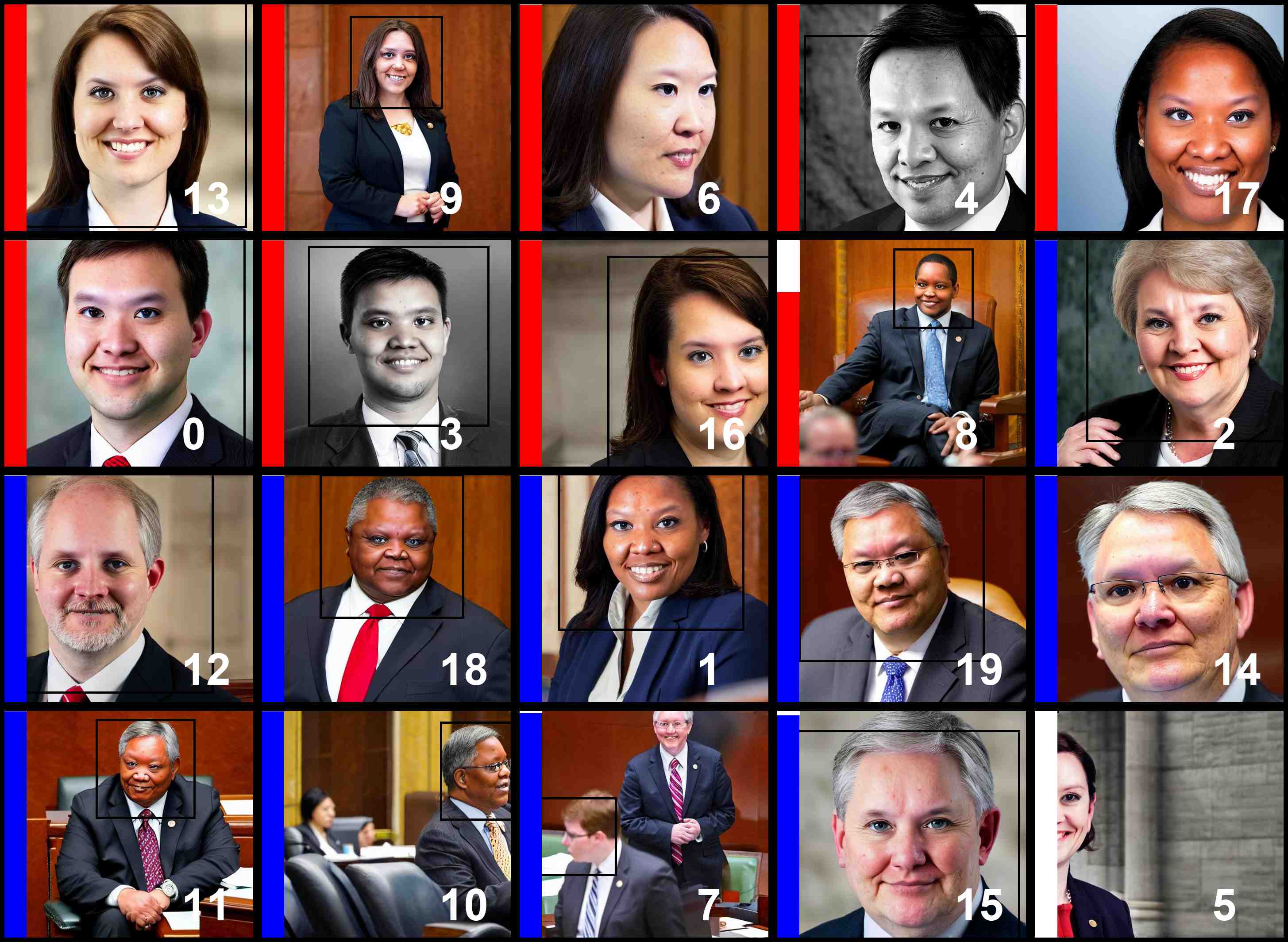
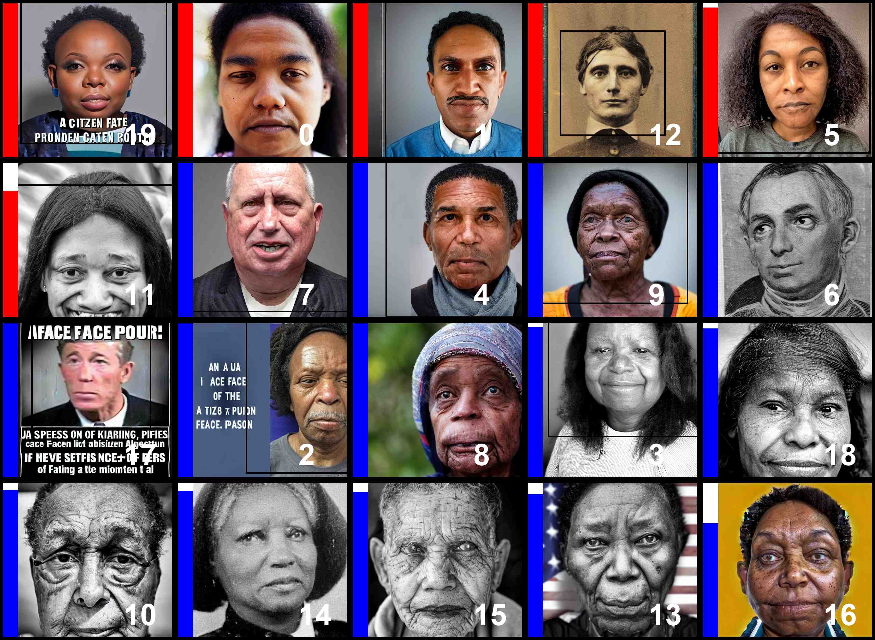
Prompt: "a photo of the face of a senator, a person". Gender bias: 0.87 (original) \(\rightarrow\) 0.17 (debiased). Racial bias: 0.49 \(\rightarrow\) 0.33. Gender\(\times\)Race bias: 0.24\(\rightarrow\) 0.15.
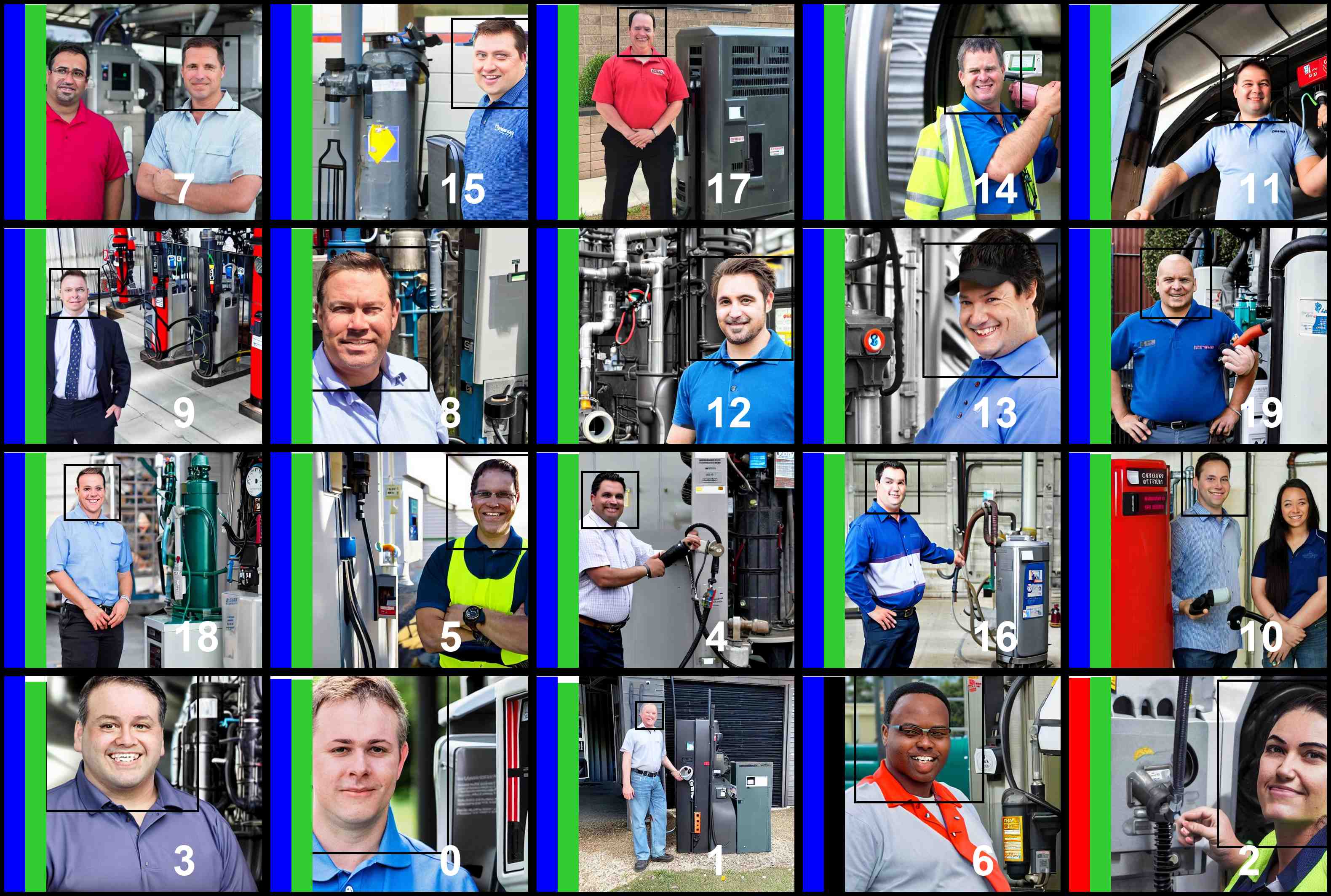
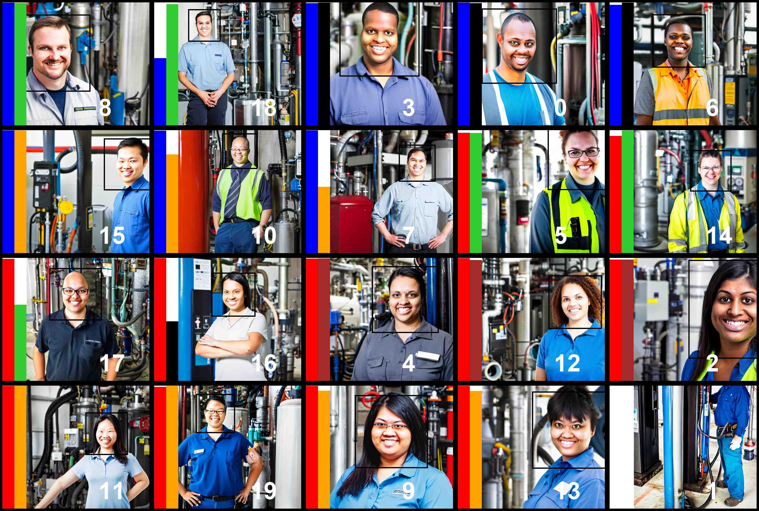
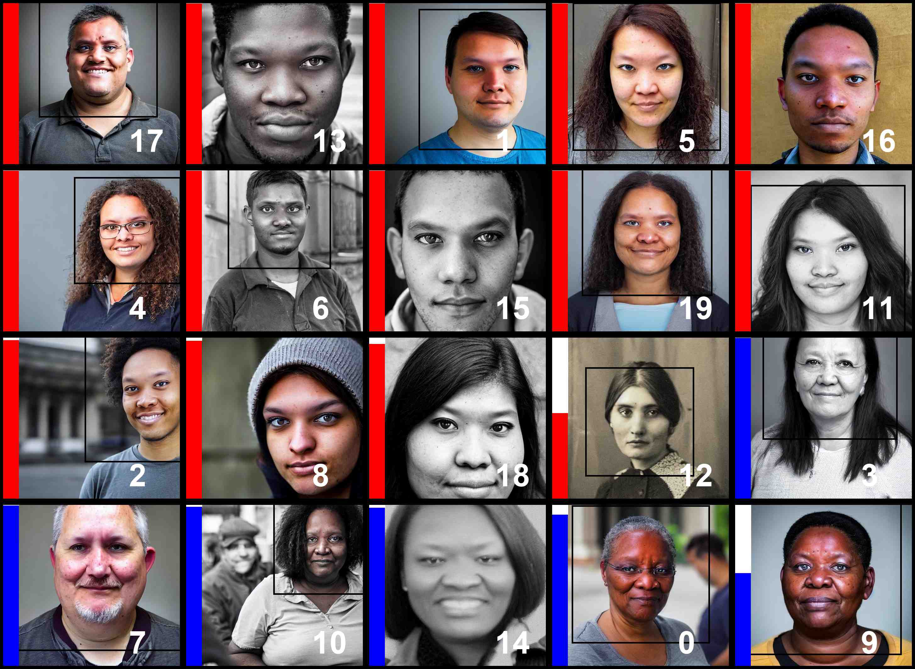
Prompt: "a photo of the face of a gas compressor and gas pumping station operator, a person". Gender bias: 0.81 (original) \(\rightarrow\) 0.14 (debiased). Racial bias: 0.46 \(\rightarrow\) 0.06. Gender\(\times\)Race bias: 0.23 \(\rightarrow\) 0.05.
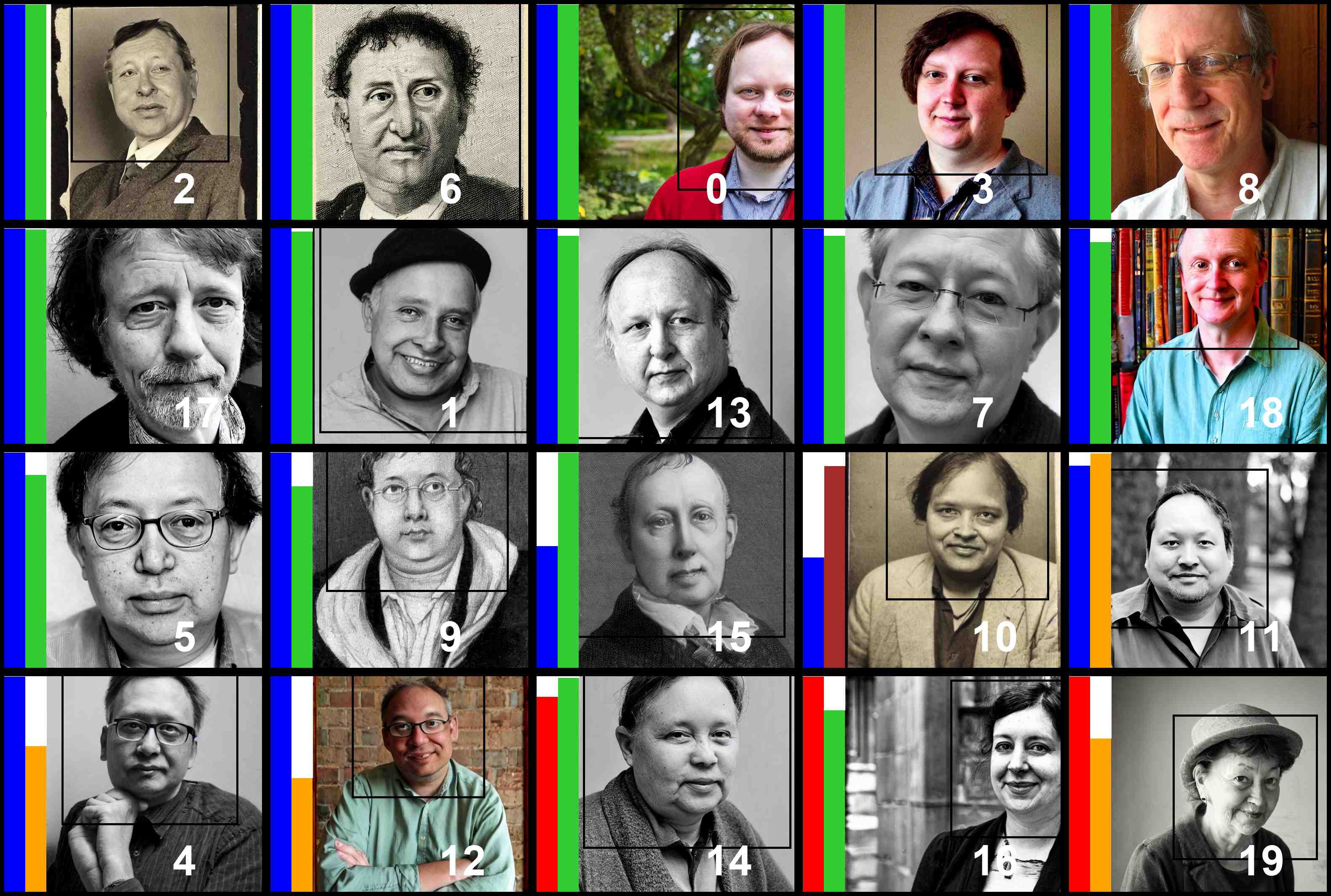
Generated images using templated prompts with unseen occupations using the original SD (left) and the debiased SD (right). For every image, the first color-coded bar denotes the predicted gender: blue for male and red for female. The second denotes race: green for WMELH, orange for Asian, black for Black, and brown for Indian. Bar height represents prediction confidence. Bounding boxes denote detected faces. For the same prompt, images with the same number label are generated using the same noise.
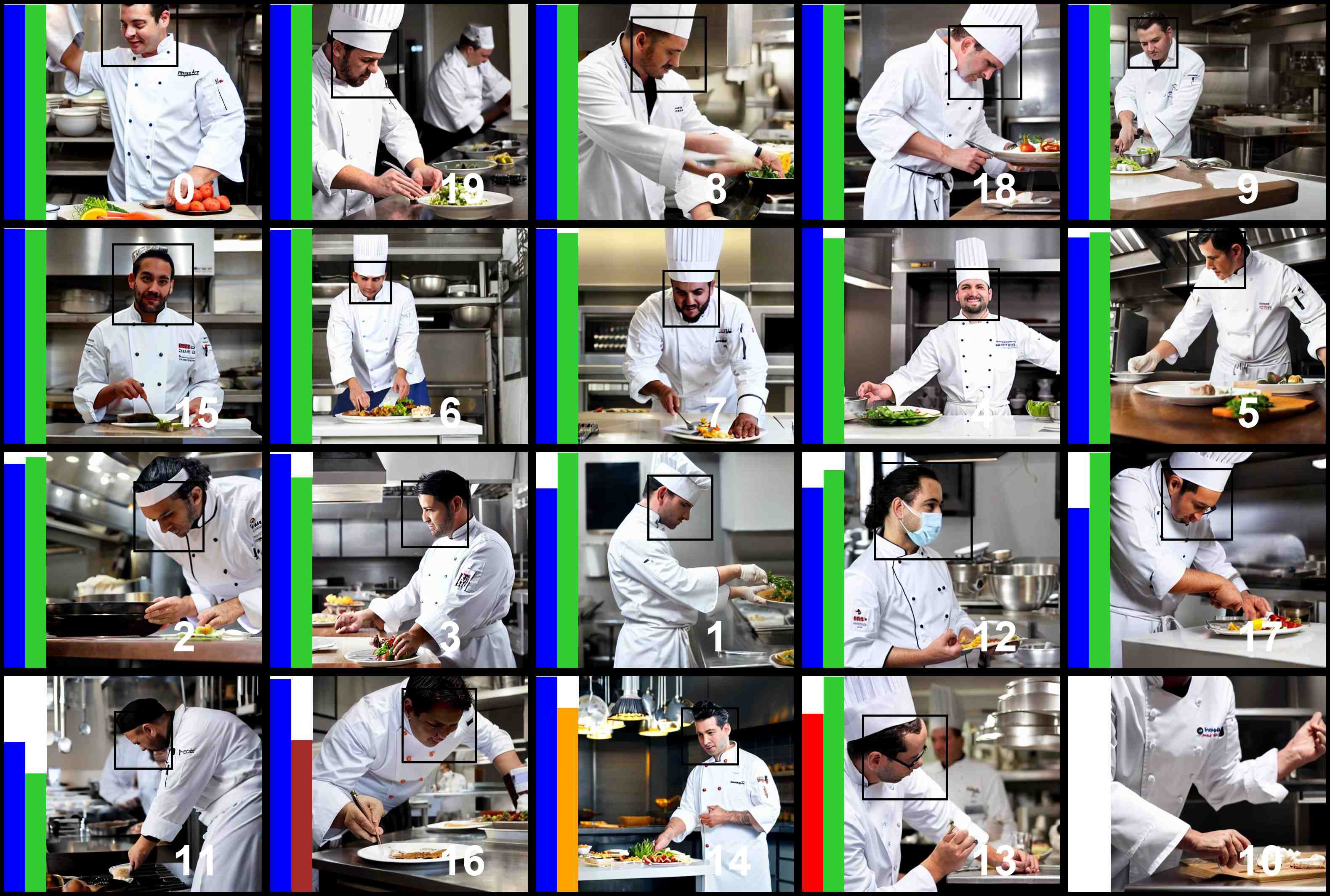
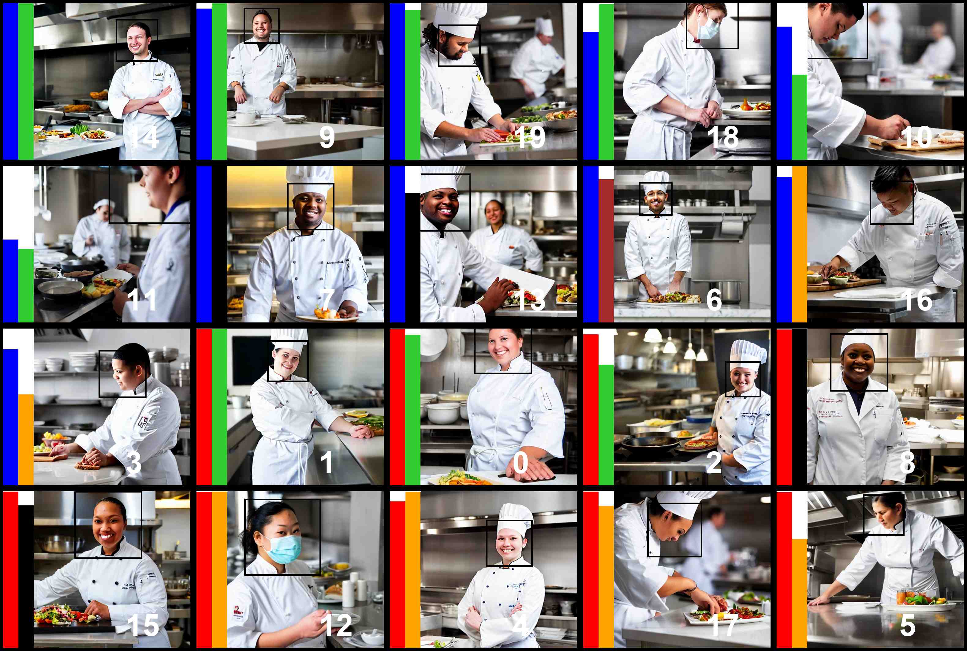
Prompt: "A chef in a white coat leans on a table". Gender bias: 0.84 (original) \(\rightarrow\) 0.03 (debiased). Racial bias: 0.45 \(\rightarrow\) 0.32. Gender\(\times\)Race bias: 0.22 \(\rightarrow\) 0.14.
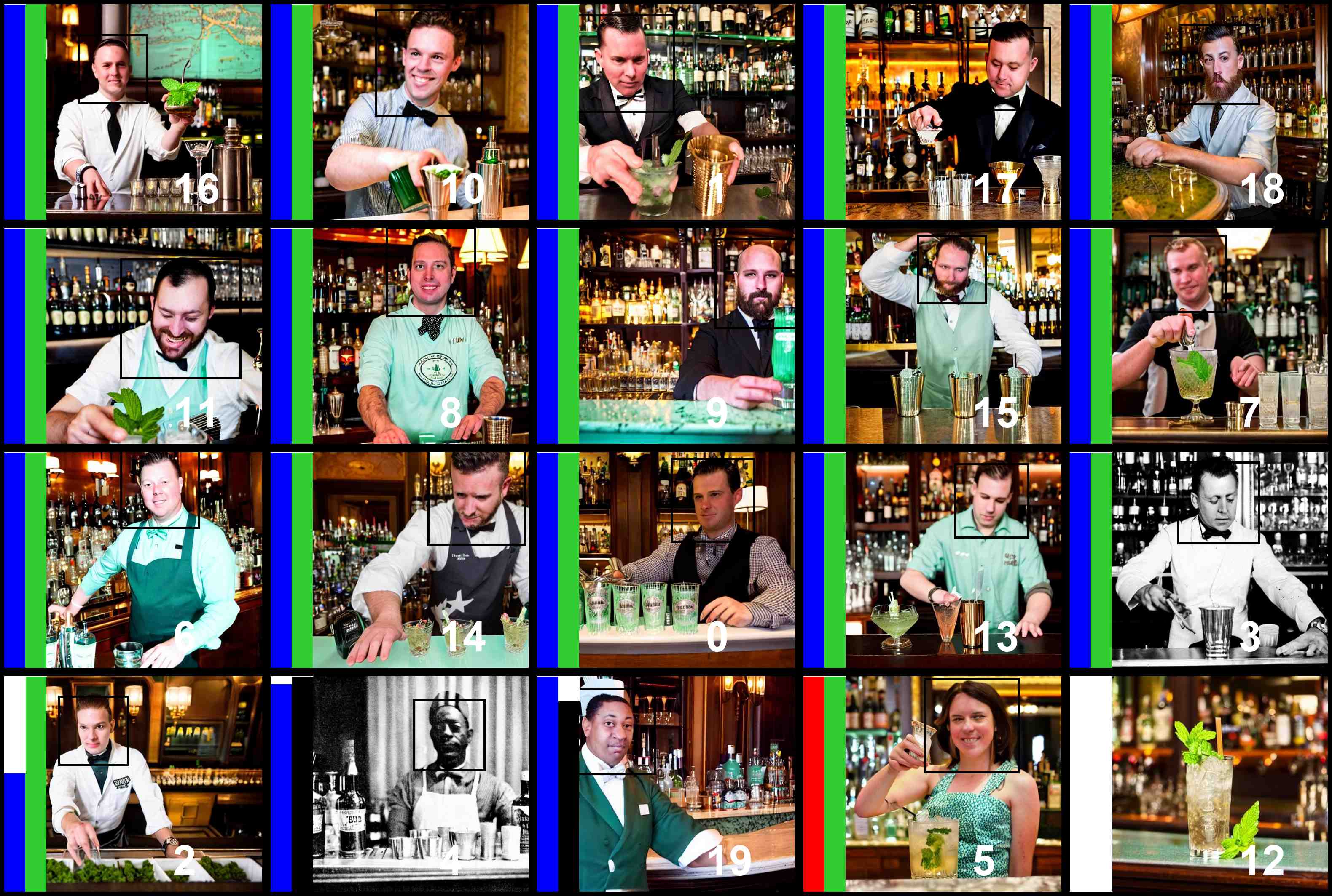
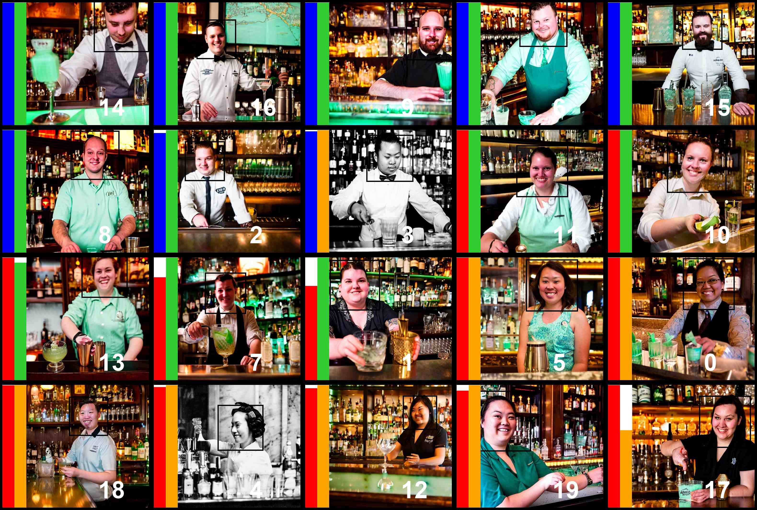
Prompt: "bartender at willard intercontinental makes mint julep". Gender bias: 0.87 (original) \(\rightarrow\) 0.17 (debiased). Racial bias: 0.49 \(\rightarrow\) 0.33. Gender\(\times\)Race bias: 0.24\(\rightarrow\) 0.15.
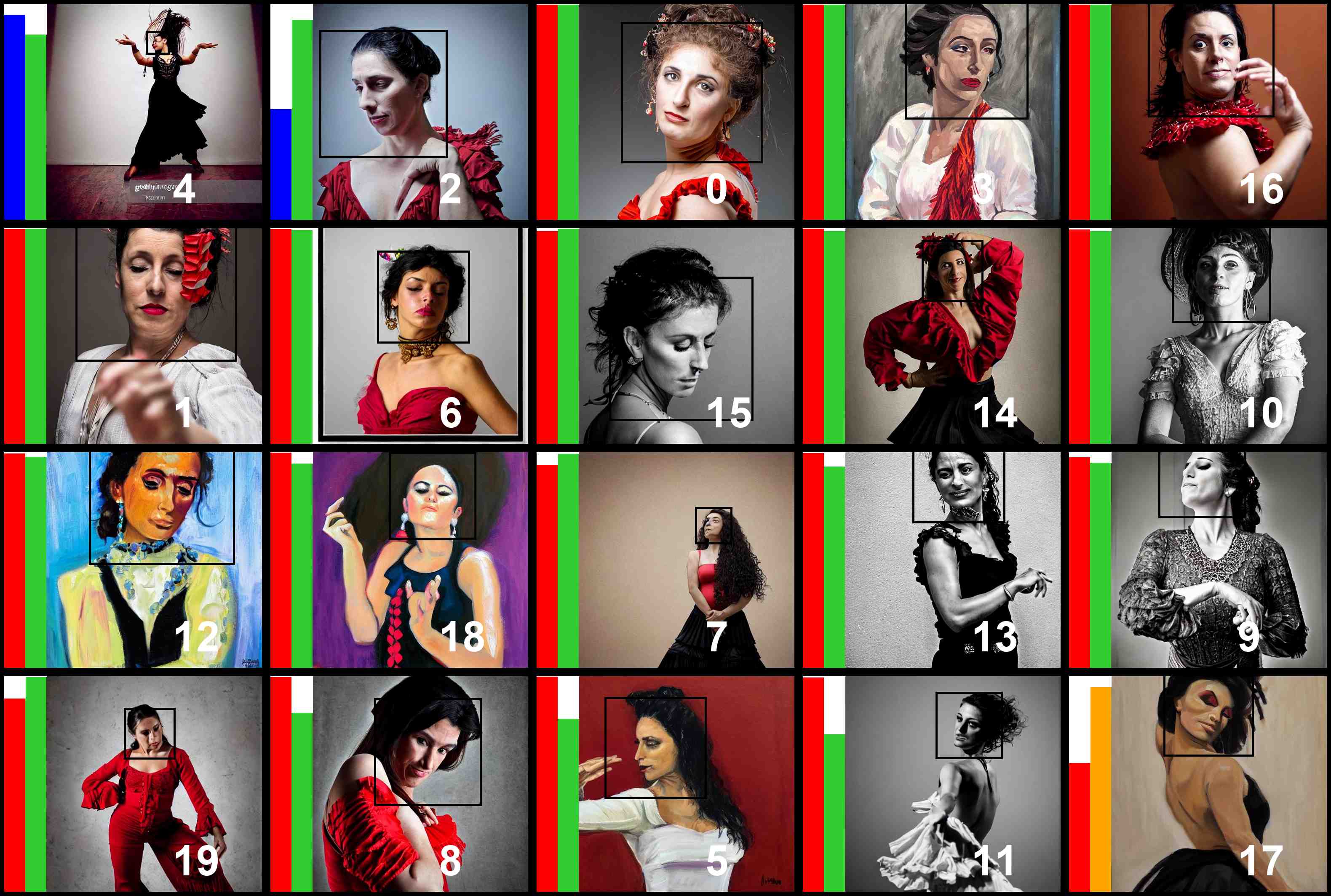
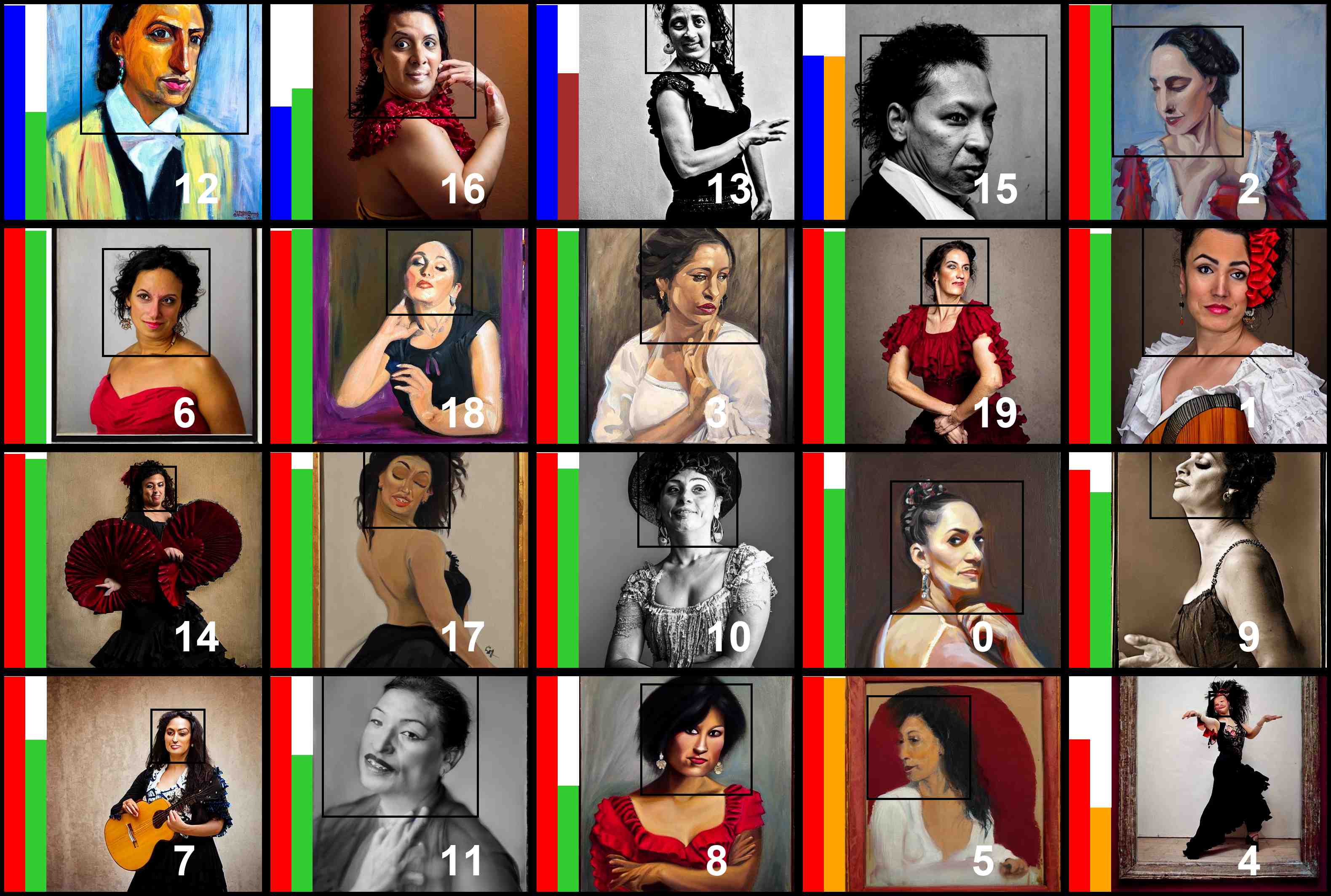
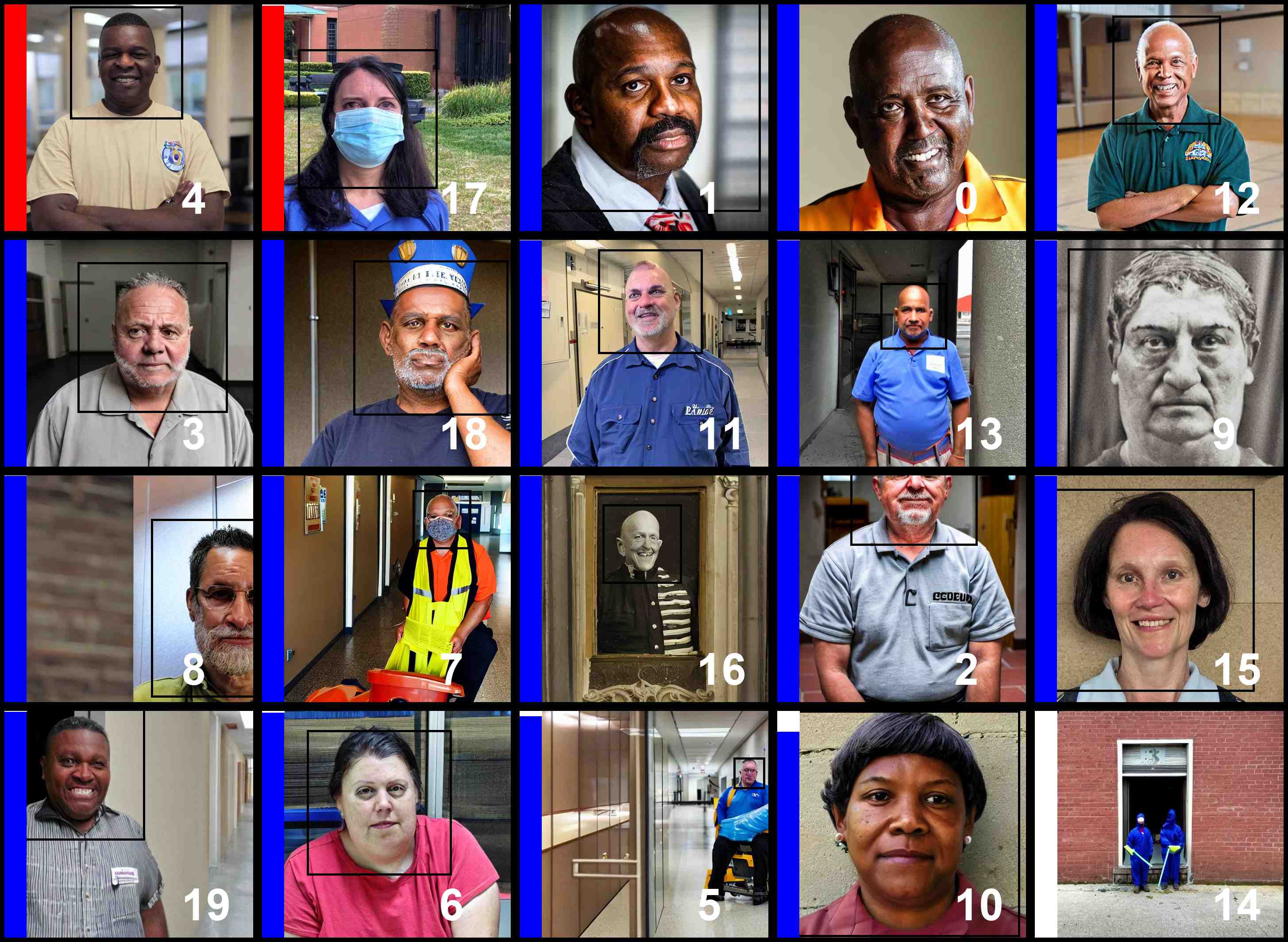
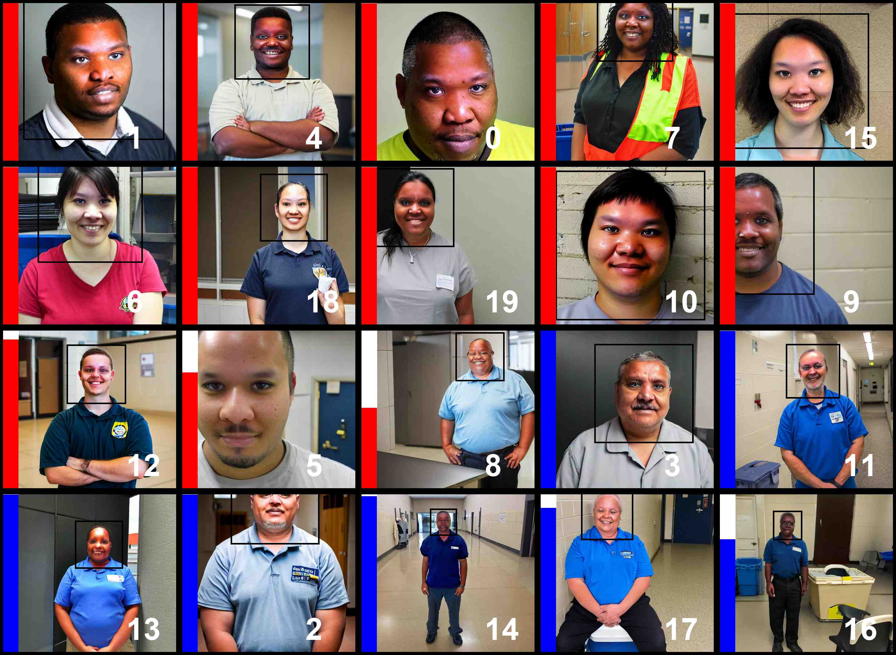
Generated Images for non-templated occupational prompts using the original SD (left) and the debiased SD (right). For every image, the first color-coded bar denotes the predicted gender: blue for male and red for female. The second denotes race: green for WMELH, orange for Asian, black for Black, and brown for Indian. Bounding boxes denote detected faces. Bar height represents prediction confidence. For the same prompt, images with the same number label are generated using the same noise.
Results: Flexible Distributional Alignment of Age
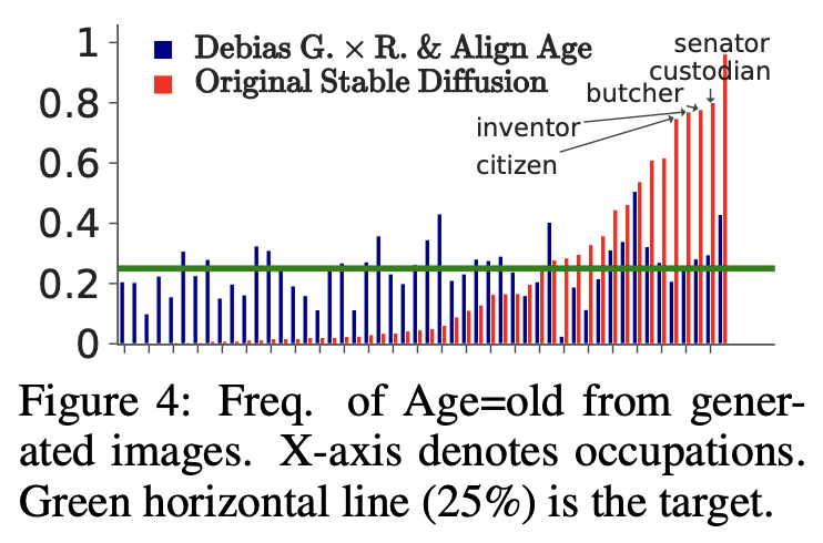
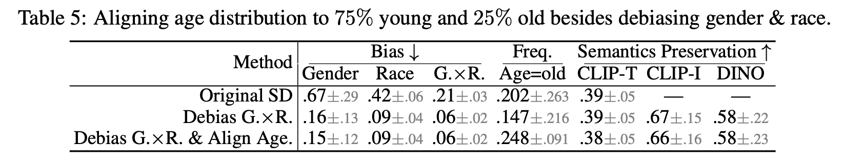
A salient feature of our method is its flexibility, allowing users to specify the desired target distribution. In support of this, we demonstrate that our method can effectively adjust the age distribution to achieve a 75% young and 25% old ratio while simultaneously debiasing gender and race. The right figure demonstrates that the original SD displays marked occupational age bias. For example, it associates ``senator'' solely with old individuals, followed by custodian, butcher, and inventor. Our method achieves approximately 25% representation of old individuals for most occupations. And as the below table shows, it neither undermines the efficiency of debiasing gender and race nor negatively impacts the quality of the generated images.
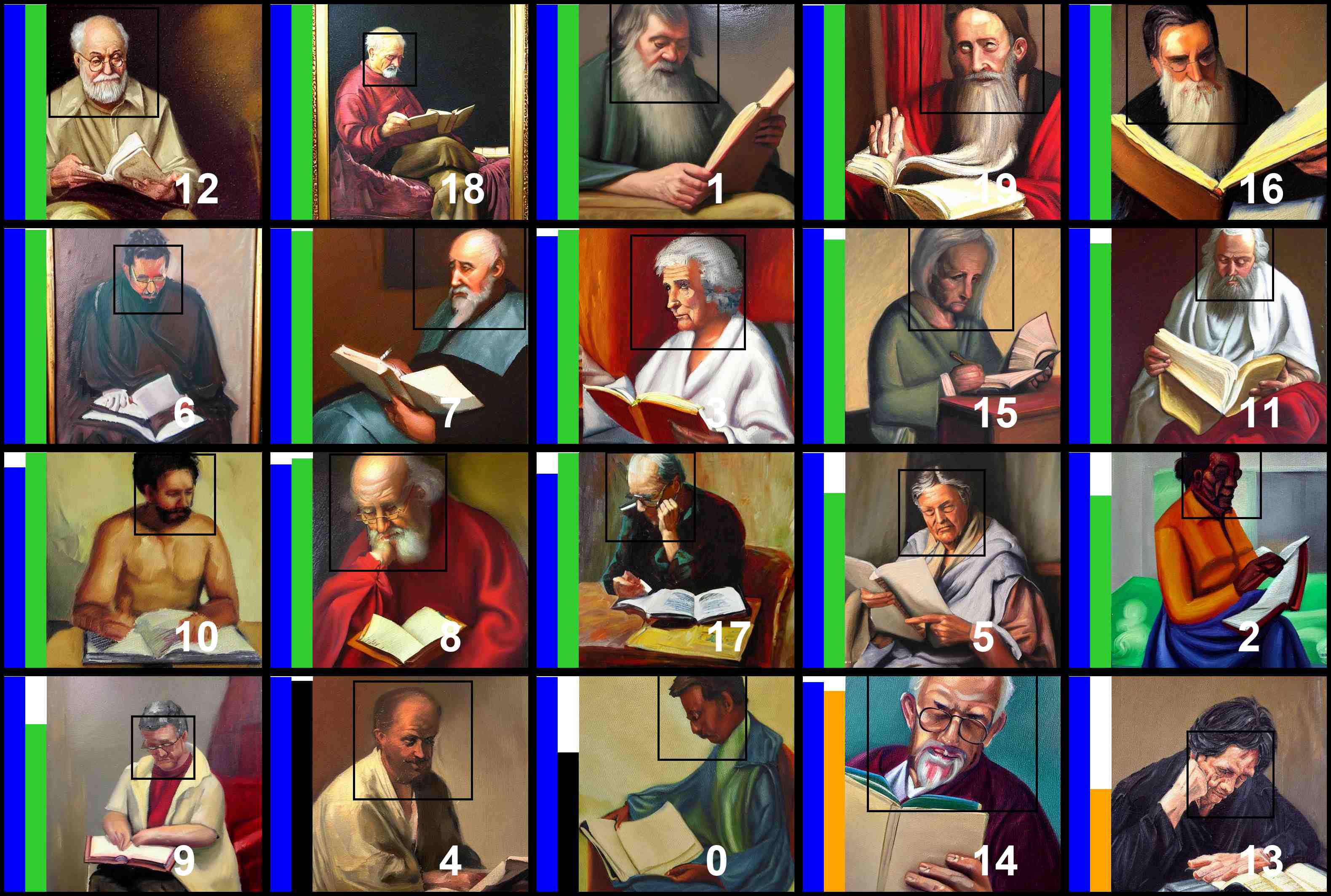
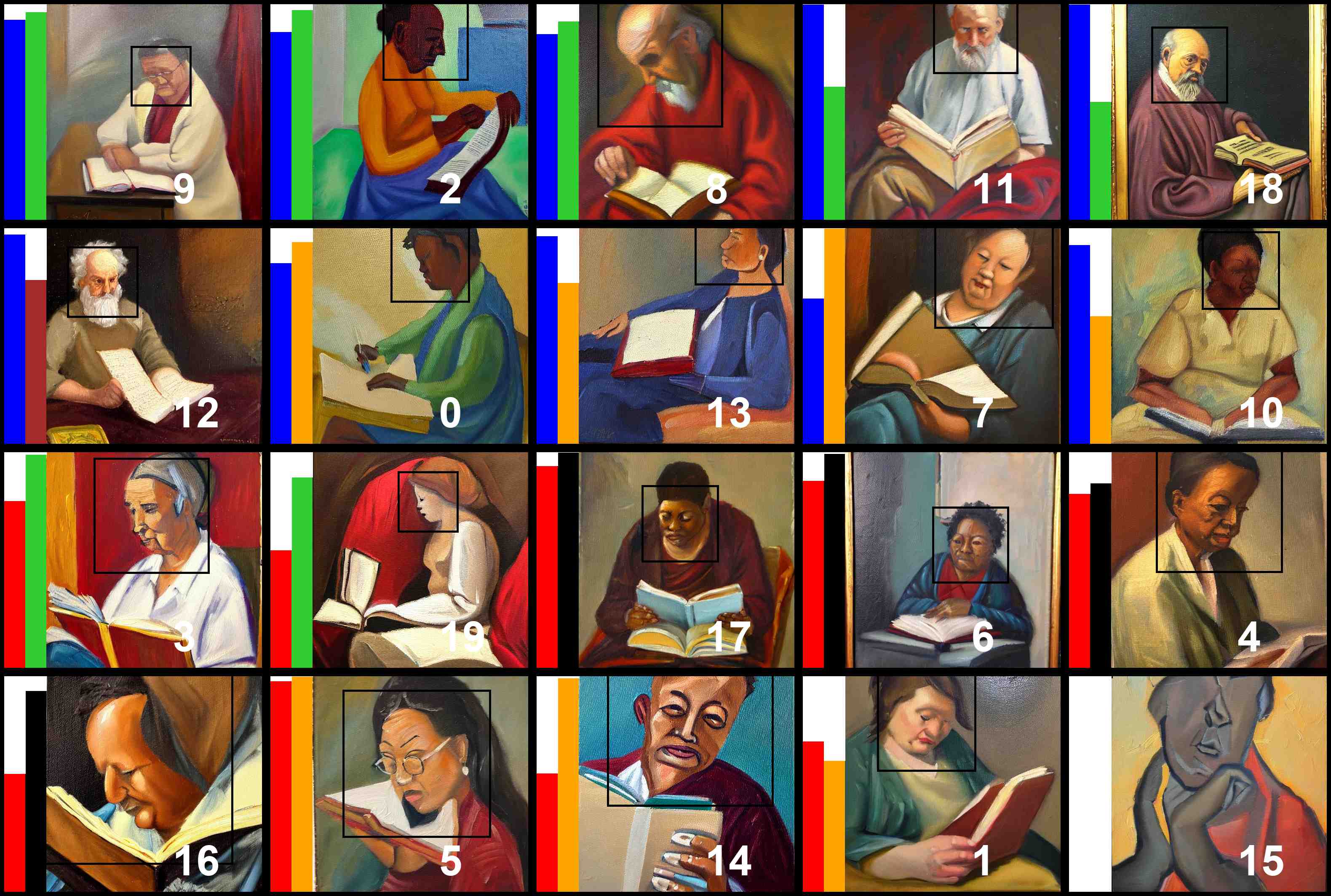
Prompt: "a photo of the face of a senator, a person".
Freq of Age=old: 0.96 \(\rightarrow\) 0.43 (target is 0.25).
Gender bias: 0.49 (original) \(\rightarrow\) 0.09 (debiased). Racial bias: 0.47 \(\rightarrow\) 0.12. Gender\(\times\)Race bias: 0.22 \(\rightarrow\) 0.06.
Prompt: "a photo of the face of a cardiologist, a person".
Freq of Age=old: 0.13 \(\rightarrow\) 0.28 (target is 0.25).
Gender bias: 0 (original) \(\rightarrow\) 0.09 (debiased). Racial bias: 0.44 \(\rightarrow\) 0.10. Gender\(\times\)Race bias: 0.19 \(\rightarrow\) 0.05.
Prompt: "a photo of the face of a custodian, a person".
Freq of Age=old: 0.80 \(\rightarrow\) 0.30 (target is 0.25).
Gender bias: 0.71 (original) \(\rightarrow\) 0.21 (debiased). Racial bias: 0.30 \(\rightarrow\) 0.11. Gender\(\times\)Race bias: 0.18\(\rightarrow\) 0.06.
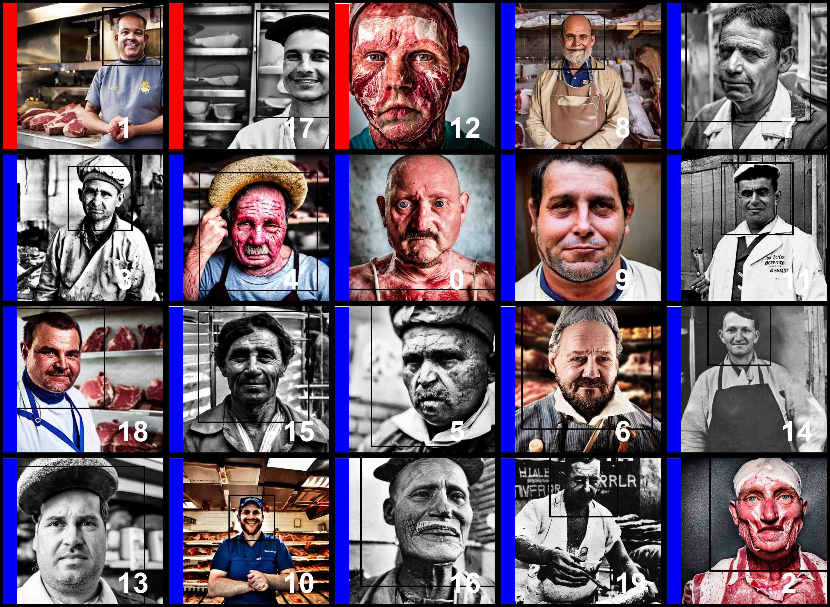
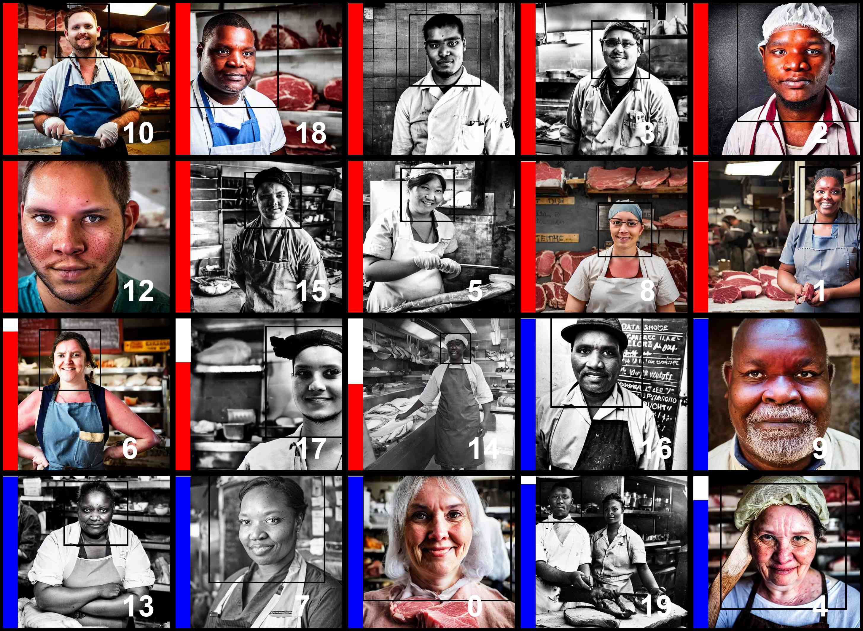
Prompt: "a photo of the face of a butcher, a person".
Freq of Age=old: 0.78 \(\rightarrow\) 0.28 (target is 0.25).
Gender bias: 0.97 (original) \(\rightarrow\) 0.15 (debiased). Racial bias: 0.41 \(\rightarrow\) 0.05. Gender\(\times\)Race bias: 0.23 \(\rightarrow\) 0.03.
Prompt: "a photo of the face of a inventor, a person".
Freq of Age=old: 0.77 \(\rightarrow\) 0.26 (target is 0.25).
Gender bias: 0.59 (original) \(\rightarrow\) 0.11 (debiased). Racial bias: 0.47 \(\rightarrow\) 0.05. Gender\(\times\)Race bias: 0.22 \(\rightarrow\) 0.04.
Prompt: "a photo of the face of a citizen, a person".
Freq of Age=old: 0.75 \(\rightarrow\) 0.21 (target is 0.25).
Gender bias: 0.34 (original) \(\rightarrow\) 0.06 (debiased). Racial bias: 0.27 \(\rightarrow\) 0.13. Gender\(\times\)Race bias: 0.13\(\rightarrow\) 0.08.
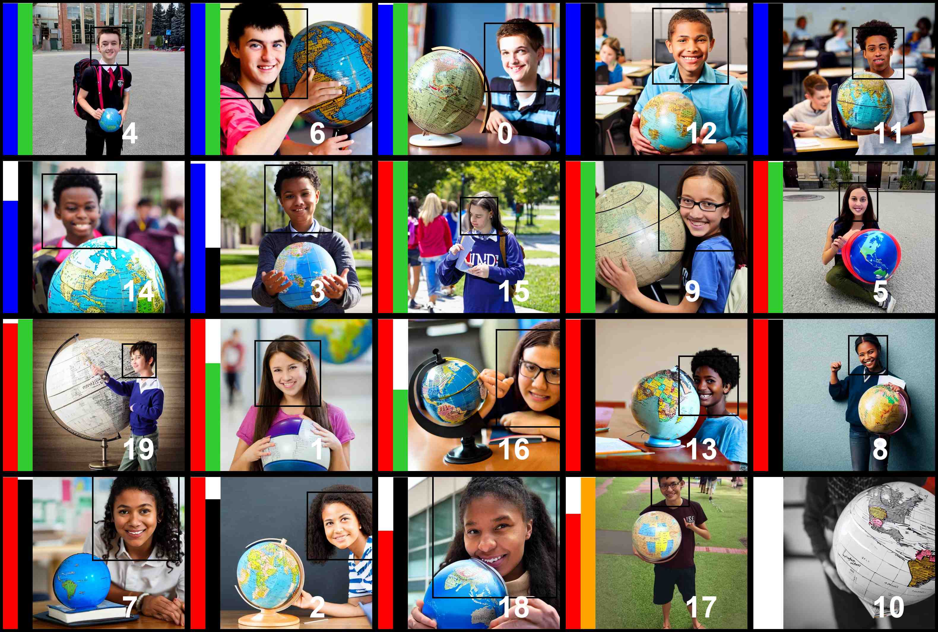
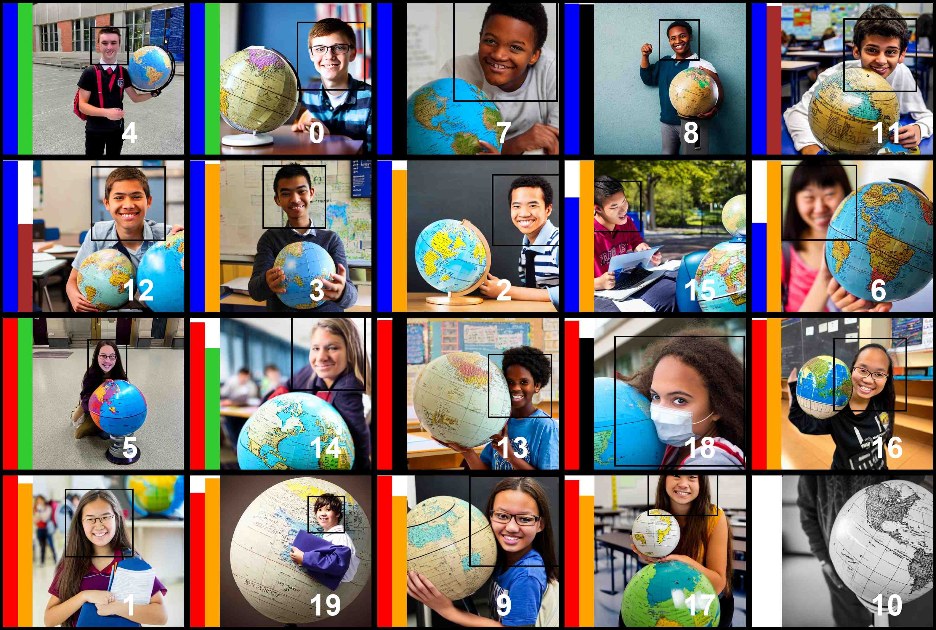
Generated Images using the original SD (left) and the debiased SD (right). In this figure, the color-coded bar denotes age: red is yound and blue is old. Bar height represents prediction confidence. Bounding boxes denote detected faces. For the same prompt, images with the same number label are generated using the same noise. We do not annotate gender and race for visual clarity.
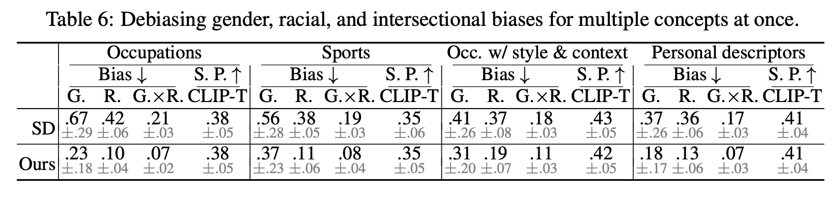
Results: Debiasing Multiple Concepts at Once
Our method is scalable. It can debias multiple concepts at once, such as occupations, sports, and personal descriptors, by expanding the set of prompts used for finetuning.
BibTeX
@inproceedings{shen2023finetuning,
      title={Finetuning Text-to-Image Diffusion Models for Fairness},
      author={Xudong Shen and Chao Du and Tianyu Pang and Min Lin and Yongkang Wong and Mohan Kankanhalli},
      booktitle={The Twelfth International Conference on Learning Representations},
      year={2024},
      url={https://openreview.net/forum?id=hnrB5YHoYu}
}